Autoencoders for Image Reconstruction in Python and Keras

Introduction

Nowadays, we have huge amounts of data in almost every application we use - listening to music on Spotify, browsing friend's images on Instagram, or maybe watching a new trailer on YouTube. There is always data being transmitted from the servers to you.

This wouldn't be a problem for a single user. But imagine handling thousands, if not millions, of requests with large data at the same time. These streams of data have to be reduced somehow in order for us to be physically able to provide them to users - this is where data compression kicks in.

There are lots of compression techniques, and they vary in their usage and compatibility. For example some compression techniques only work on audio files, like the famous MPEG-2 Audio Layer III (MP3) codec.

There are two main types of compression:

• Lossless: Data integrity and accuracy is preferred, even if we don't "shave off" much
• Lossy: Data integrity and accuracy isn't as important as how fast we can serve it - imagine a real-time video transfer, where it's more important to be "live" than to have high quality video

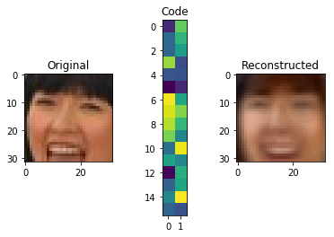
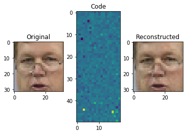
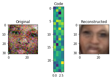
For example, using Autoencoders, we're able to decompose this image and represent it as the 32-vector code below. Using it, we can reconstruct the image. Of course, this is an example of lossy compression, as we've lost quite a bit of info.

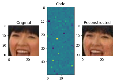
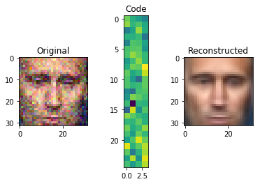
Though, we can use the exact same technique to do this much more accurately, by allocating more space for the representation:

What are Autoencoders?

An autoencoder is, by definition, a technique to encode something automatically. By using a neural network, the autoencoder is able to learn how to decompose data (in our case, images) into fairly small bits of data, and then using that representation, reconstruct the original data as closely as it can to the original.

There are two key components in this task:

• Encoder: Learns how to compress the original input into a small encoding
• Decoder: Learns how to restore the original data from that encoding generated by the Encoder

These two are trained together in symbiosis to obtain the most efficient representation of the data that we can reconstruct the original data from, without losing so much of it.

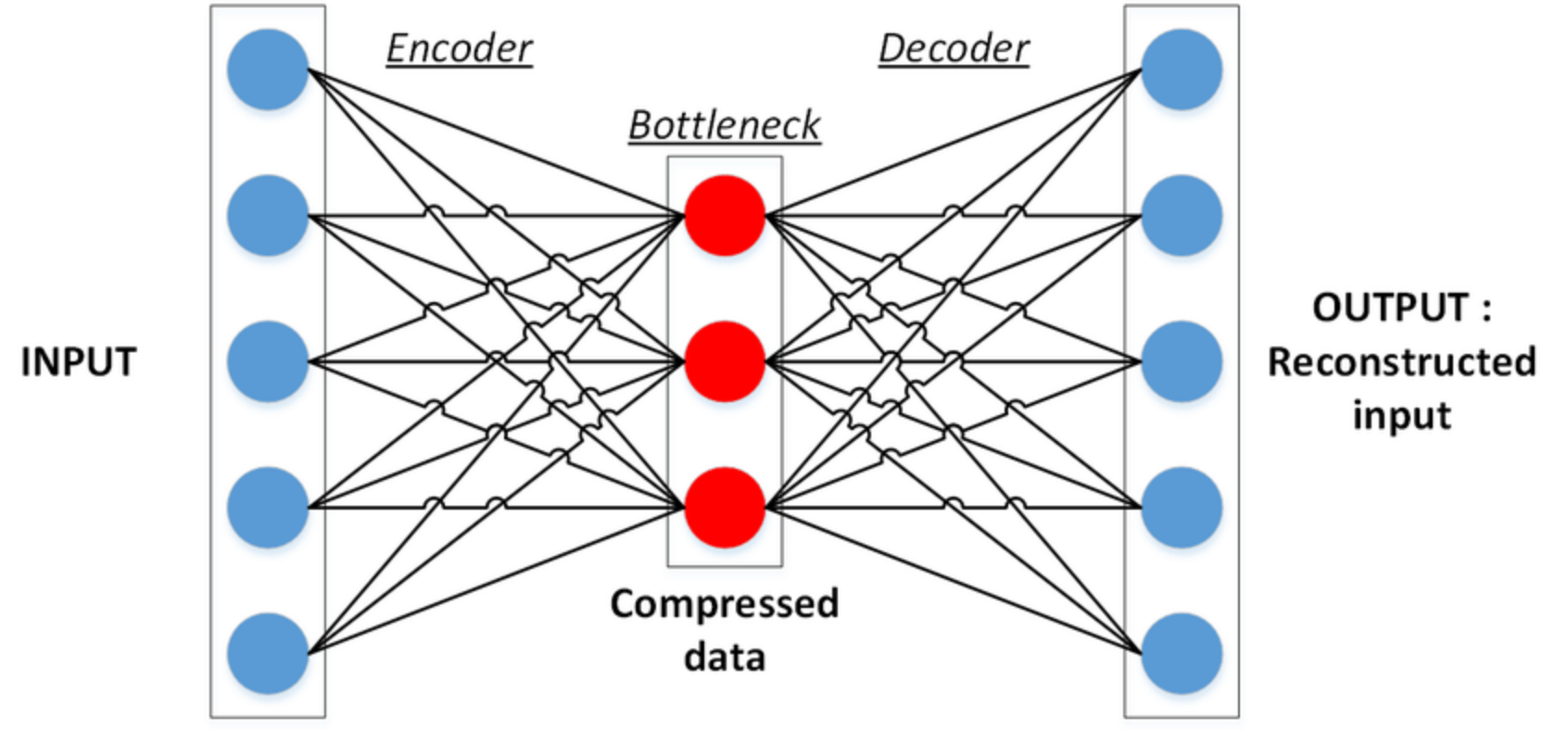
Credit: ResearchGate

Encoder

The Encoder is tasked with finding the smallest possible representation of data that it can store - extracting the most prominent features of the original data and representing it in a way the decoder can understand.

Think of it as if you are trying to memorize something, like for example memorizing a large number - you try to find a pattern in it that you can memorize and restore the whole sequence from that pattern, as it will be easy to remember a shorter pattern than the whole number.

Encoders in their simplest form are simple Artificial Neural Networks (ANNs). Though, there are certain encoders that utilize Convolutional Neural Networks (CNNs), which is a very specific type of ANN.

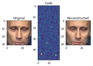
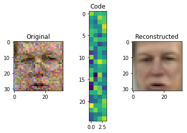
The encoder takes the input data and generates an encoded version of it - the compressed data. We can then use that compressed data to send it to the user, where it will be decoded and reconstructed. Let's take a look at the encoding for a LFW dataset example:

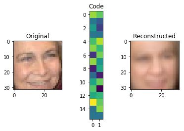
The encoding here doesn't make much sense for us, but it's plenty enough for the decoder. Now, it's valid to raise the question:

"But how did the encoder learn to compress images like this?

This is where the symbiosis during training comes into play.

Decoder

The Decoder works in a similar way to the encoder, but the other way around. It learns to read, instead of generate, these compressed code representations and generate images based on that info. It aims to minimize the loss while reconstructing, obviously.

The output is evaluated by comparing the reconstructed image by the original one, using a Mean Square Error (MSE) - the more similar it is to the original, the smaller the error.

At this point, we propagate backwards and update all the parameters from the decoder to the encoder. Therefore, based on the differences between the input and output images, both the decoder and encoder get evaluated at their jobs and update their parameters to become better.

Building an Autoencoder

Keras is a Python framework that makes building neural networks simpler. It allows us to stack layers of different types to create a deep neural network - which we will do to build an autoencoder.

First, let's install Keras using pip:

$ pip install keras

Preprocessing Data

Again, we'll be using the LFW dataset. As usual, with projects like these, we'll preprocess the data to make it easier for our autoencoder to do its job.

For this, we'll first define a couple of paths which lead to the dataset we're using:

# http://www.cs.columbia.edu/CAVE/databases/pubfig/download/lfw_attributes.txt
ATTRS_NAME = "lfw_attributes.txt"

# http://vis-www.cs.umass.edu/lfw/lfw-deepfunneled.tgz
IMAGES_NAME = "lfw-deepfunneled.tgz"

# http://vis-www.cs.umass.edu/lfw/lfw.tgz
RAW_IMAGES_NAME = "lfw.tgz"

Then, we'll employ two functions - one to convert the raw matrix into an image and change the color system to RGB:

def decode_image_from_raw_bytes(raw_bytes):
    img = cv2.imdecode(np.asarray(bytearray(raw_bytes), dtype=np.uint8), 1)
    img = cv2.cvtColor(img, cv2.COLOR_BGR2RGB)
    return img

And the other one to actually load the dataset and adapt it to our needs:

def load_lfw_dataset(
        use_raw=False,
        dx=80, dy=80,
        dimx=45, dimy=45):

    # Read attrs
    df_attrs = pd.read_csv(ATTRS_NAME, sep='\t', skiprows=1)
    df_attrs = pd.DataFrame(df_attrs.iloc[:, :-1].values, columns=df_attrs.columns[1:])
    imgs_with_attrs = set(map(tuple, df_attrs[["person", "imagenum"]].values))

    # Read photos
    all_photos = []
    photo_ids = []

    # tqdm in used to show progress bar while reading the data in a notebook here, you can change
    # tqdm_notebook to use it outside a notebook
    with tarfile.open(RAW_IMAGES_NAME if use_raw else IMAGES_NAME) as f:
        for m in tqdm.tqdm_notebook(f.getmembers()):
            # Only process image files from the compressed data
            if m.isfile() and m.name.endswith(".jpg"):
                # Prepare image
                img = decode_image_from_raw_bytes(f.extractfile(m).read())

                # Crop only faces and resize it
                img = img[dy:-dy, dx:-dx]
                img = cv2.resize(img, (dimx, dimy))

                # Parse person and append it to the collected data
                fname = os.path.split(m.name)[-1]
                fname_splitted = fname[:-4].replace('_', ' ').split()
                person_id = ' '.join(fname_splitted[:-1])
                photo_number = int(fname_splitted[-1])
                if (person_id, photo_number) in imgs_with_attrs:
                    all_photos.append(img)
                    photo_ids.append({'person': person_id, 'imagenum': photo_number})

    photo_ids = pd.DataFrame(photo_ids)
    all_photos = np.stack(all_photos).astype('uint8')

    # Preserve photo_ids order!
    all_attrs = photo_ids.merge(df_attrs, on=('person', 'imagenum')).drop(["person", "imagenum"], axis=1)

    return all_photos, all_attrs

Implementing the Autoencoder

import numpy as np
X, attr = load_lfw_dataset(use_raw=True, dimx=32, dimy=32)

Our data is in the X matrix, in the form of a 3D matrix, which is the default representation for RGB images. By providing three matrices - red, green, and blue, the combination of these three generate the image color.

These images will have large values for each pixel, ranging from 0 to 255. Generally in machine learning we tend to make values small, and centered around 0, as this helps our model train faster and get better results, so let's normalize our images:

X = X.astype('float32') / 255.0 - 0.5

By now if we test the X array for the min and max it will be -.5 and .5, which you can verify:

print(X.max(), X.min())

0.5 -0.5

To be able to see the image, let's create a show_image function. It will add 0.5 to the images as the pixel value can't be negative:

import matplotlib.pyplot as plt
def show_image(x):
    plt.imshow(np.clip(x + 0.5, 0, 1))

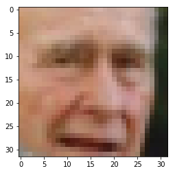
Now let's take a quick look at our data:

show_image(X[6])

Great, now let's split our data into a training and test set:

from sklearn.model_selection import train_test_split
X_train, X_test = train_test_split(X, test_size=0.1, random_state=42)

The sklearn train_test_split() function is able to split the data by giving it the test ratio and the rest is, of course, the training size. The random_state, which you are going to see a lot in machine learning, is used to produce the same results no matter how many times you run the code.

Now time for the model:

from keras.layers import Dense, Flatten, Reshape, Input, InputLayer
from keras.models import Sequential, Model

def build_autoencoder(img_shape, code_size):
    # The encoder
    encoder = Sequential()
    encoder.add(InputLayer(img_shape))
    encoder.add(Flatten())
    encoder.add(Dense(code_size))

    # The decoder
    decoder = Sequential()
    decoder.add(InputLayer((code_size,)))
    decoder.add(Dense(np.prod(img_shape))) # np.prod(img_shape) is the same as 32*32*3, it's more generic than saying 3072
    decoder.add(Reshape(img_shape))

    return encoder, decoder

This function takes an image_shape (image dimensions) and code_size (the size of the output representation) as parameters. The image shape, in our case, will be (32, 32, 3) where 32 represents the width and height, and 3 represents the color channel matrices. That being said, our image has 3072 dimensions.

Logically, the smaller the code_size is, the more the image will compress, but fewer features will be saved and the reproduced image will be that much more different from the original.

A Keras sequential model is basically used to sequentially add layers and deepen our network. Each layer feeds into the next one, and here, we're simply starting off with the InputLayer (a placeholder for the input) with the size of the input vector - image_shape.

The Flatten layer's job is to flatten the (32,32,3) matrix into a 1D array (3072) since the network architecture doesn't accept 3D matrices.

The last layer in the encoder is the Dense layer, which is the actual neural network here. It tries to find the optimal parameters that achieve the best output - in our case it's the encoding, and we will set the output size of it (also the number of neurons in it) to the code_size.

The decoder is also a sequential model. It accepts the input (the encoding) and tries to reconstruct it in the form of a row. Then, it stacks it into a 32x32x3 matrix through the Dense layer. The final Reshape layer will reshape it into an image.

Now let's connect them together and start our model:

# Same as (32,32,3), we neglect the number of instances from shape
IMG_SHAPE = X.shape[1:]
encoder, decoder = build_autoencoder(IMG_SHAPE, 32)

inp = Input(IMG_SHAPE)
code = encoder(inp)
reconstruction = decoder(code)

autoencoder = Model(inp,reconstruction)
autoencoder.compile(optimizer='adamax', loss='mse')

print(autoencoder.summary())

This code is pretty straightforward - our code variable is the output of the encoder, which we put into the decoder and generate the reconstruction variable.

Afterwards, we link them both by creating a Model with the inp and reconstruction parameters and compile them with the adamax optimizer and mse loss function.

Compiling the model here means defining its objective and how to reach it. The objective in our context is to minimize the mse and we reach that by using an optimizer - which is basically a tweaked algorithm to find the global minimum.

At this point, we can summarize the results:

_________________________________________________________________
Layer (type)                 Output Shape              Param #
=================================================================
input_6 (InputLayer)         (None, 32, 32, 3)         0
_________________________________________________________________
sequential_3 (Sequential)    (None, 32)                98336
_________________________________________________________________
sequential_4 (Sequential)    (None, 32, 32, 3)         101376
=================================================================
Total params: 199,712
Trainable params: 199,712
Non-trainable params: 0
_________________________________________________________________

Here we can see the input is 32,32,3. Note the None here refers to the instance index, as we give the data to the model it will have a shape of (m, 32,32,3), where m is the number of instances, so we keep it as None.

The hidden layer is 32, which is indeed the encoding size we chose, and lastly the decoder output as you see is (32,32,3).

Now, let's trade the model:

history = autoencoder.fit(x=X_train, y=X_train, epochs=20,
                validation_data=[X_test, X_test])

In our case, we'll be comparing the constructed images to the original ones, so both x and y are equal to X_train. Ideally, the input is equal to the output.

The epochs variable defines how many times we want the training data to be passed through the model and the validation_data is the validation set we use to evaluate the model after training:

Train on 11828 samples, validate on 1315 samples
Epoch 1/20
11828/11828 [==============================] - 3s 272us/step - loss: 0.0128 - val_loss: 0.0087
Epoch 2/20
11828/11828 [==============================] - 3s 227us/step - loss: 0.0078 - val_loss: 0.0071
.
.
.
Epoch 20/20
11828/11828 [==============================] - 3s 237us/step - loss: 0.0067 - val_loss: 0.0066

We can visualize the loss over epochs to get an overview about the epochs number.

plt.plot(history.history['loss'])
plt.plot(history.history['val_loss'])
plt.title('model loss')
plt.ylabel('loss')
plt.xlabel('epoch')
plt.legend(['train', 'test'], loc='upper left')
plt.show()

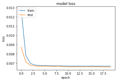
We can see that after the third epoch, there's no significant progress in loss. Visualizing like this can help you get a better idea of how many epochs is really enough to train your model. In this case, there's simply no need to train it for 20 epochs, and most of the training is redundant.

This can also lead to overfitting the model, which will make it perform poorly on new data outside the training and testing datasets.

Now, the most anticipated part - let's visualize the results:

def visualize(img,encoder,decoder):
    """Draws original, encoded and decoded images"""
    # img[None] will have shape of (1, 32, 32, 3) which is the same as the model input
    code = encoder.predict(img[None])[0]
    reco = decoder.predict(code[None])[0]

    plt.subplot(1,3,1)
    plt.title("Original")
    show_image(img)

    plt.subplot(1,3,2)
    plt.title("Code")
    plt.imshow(code.reshape([code.shape[-1]//2,-1]))

    plt.subplot(1,3,3)
    plt.title("Reconstructed")
    show_image(reco)
    plt.show()

for i in range(5):
    img = X_test[i]
    visualize(img,encoder,decoder)

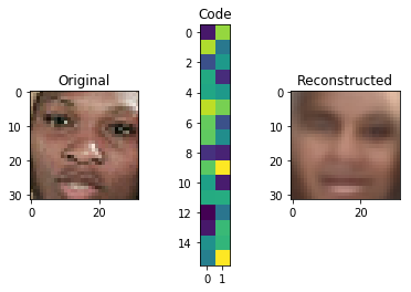
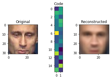
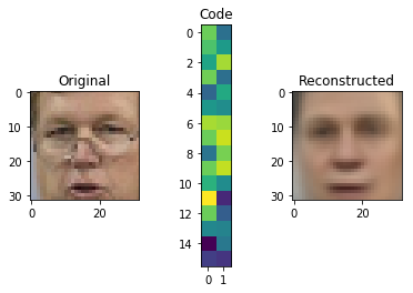
You can see that the results are not really good. However, if we take into consideration that the whole image is encoded in the extremely small vector of 32 seen in the middle, this isn't bad at all. Through the compression from 3072 dimensions to just 32 we lose a lot of data.

Now, let's increase the code_size to 1000:

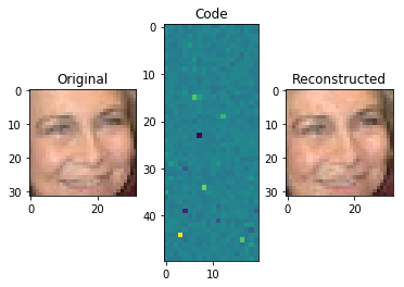
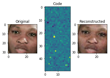
See the difference? As you give the model more space to work with, it saves more important information about the image

Note: The encoding is not two-dimensional, as represented above. This is just for illustration purposes. In reality, it's a one dimensional array of 1000 dimensions.

What we just did is called Principal Component Analysis (PCA), which is a dimensionality reduction technique. We can use it to reduce the feature set size by generating new features that are smaller in size, but still capture the important information.

Principal component analysis is a very popular usage of autoencoders.

Image De-noising

Another popular usage of autoencoders is de-noising. Let's add some random noise to our pictures:

def apply_gaussian_noise(X, sigma=0.1):
    noise = np.random.normal(loc=0.0, scale=sigma, size=X.shape)
    return X + noise

Here we add some random noise from standard normal distribution with a scale of sigma, which defaults to 0.1.

For reference, this is what noise looks like with different sigma values:

plt.subplot(1,4,1)
show_image(X_train[0])
plt.subplot(1,4,2)
show_image(apply_gaussian_noise(X_train[:1],sigma=0.01)[0])
plt.subplot(1,4,3)
show_image(apply_gaussian_noise(X_train[:1],sigma=0.1)[0])
plt.subplot(1,4,4)
show_image(apply_gaussian_noise(X_train[:1],sigma=0.5)[0])

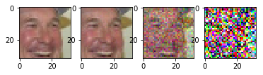
As we can see, as sigma increases to 0.5 the image is barely seen. We will try to regenerate the original image from the noisy ones with a sigma of 0.1.

The model we'll be generating for this is the same as the one from before, though we'll train it differently. This time around, we'll train it with the original and corresponding noisy images:

code_size = 100

# We can use bigger code size for better quality
encoder, decoder = build_autoencoder(IMG_SHAPE, code_size=code_size)

inp = Input(IMG_SHAPE)
code = encoder(inp)
reconstruction = decoder(code)

autoencoder = Model(inp, reconstruction)
autoencoder.compile('adamax', 'mse')

for i in range(25):
    print("Epoch %i/25, Generating corrupted samples..."%(i+1))
    X_train_noise = apply_gaussian_noise(X_train)
    X_test_noise = apply_gaussian_noise(X_test)

    # We continue to train our model with new noise-augmented data
    autoencoder.fit(x=X_train_noise, y=X_train, epochs=1,
                    validation_data=[X_test_noise, X_test])

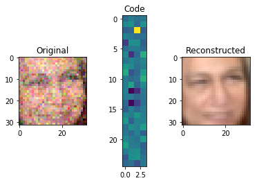
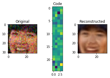
Now let's see the model results:

X_test_noise = apply_gaussian_noise(X_test)
for i in range(5):
    img = X_test_noise[i]
    visualize(img,encoder,decoder)

Autoencoder Applications

There are many more usages for autoencoders, besides the ones we've explored so far.

Autoencoder can be used in applications like Deepfakes, where you have an encoder and decoder from different models.

For example, let's say we have two autoencoders for Person X and one for Person Y. There's nothing stopping us from using the encoder of Person X and the decoder of Person Y and then generate images of Person Y with the prominent features of Person X:

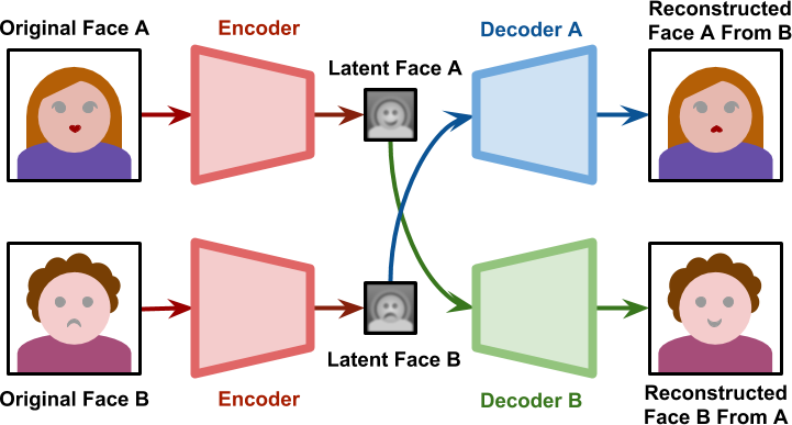
Credit: AlanZucconi

Autoencoders can also used for image segmentation - like in autonomous vehicles where you need to segment different items for the vehicle to make a decision:

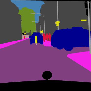
Credit: PapersWithCode

Conclusion

Autoencoders can be used for Principal Component Analysis which is a dimensionality reduction technique, image de-noising and much more.

You can try it yourself with different dataset, like for example the MNIST dataset and see what results you get.