A* Search Algorithm


What is A*?
Let's say that you have to get through an enormous maze. This maze is so big that it would take hours to find the goal manually. Additionally, once you finish the maze "by foot", you're supposed to finish another one.
To make things significantly easier and less time consuming, we'll boil the maze down to a search problem, and come up with a solution that can be applied to any additional maze that we may encounter - as long as it follows the same rules/structure.
Any time we want to convert any kind of problem into a search problem, we have to define six things:
- A set of all states we might end up in
- The start and finish state
- A finish check (a way to check if we're at the finished state)
- A set of possible actions (in this case, different directions of movement)
- A traversal function (a function that will tell us where we'll end up if we go a certain direction)
- A set of movement costs from state-to-state (which correspond to edges in the graph)
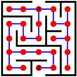
The maze problem can be solved by mapping the intersections to appropriate nodes (red dots), and the possible directions we can go to appropriate graph edges (blue lines).
Naturally, we define the start and finish states as the intersections where we enter the maze (node A), and where we want to exit the maze (node B).
Now that we have a finished graph, we can discuss algorithms for finding a path from state A to state B. In simple cases (like this one), where the generated graph consists of a small number of nodes and edges, BFS, DFS and Dijkstra would suffice.
However, in a real-life scenario, because we are dealing with problems of enormous combinatorial complexity, we know we will have to deal with an enormous amount of nodes and edges. For example, there are many states a Rubik's cube can be in, which is why solving it is so difficult. Therefore, we have to use an algorithm that is, in a sense, guided. That is where an informed search algorithm arises, A*.
Informed Search signifies that the algorithm has extra information, to begin with. For example, an uninformed search problem algorithm would be finding a path from home to work completely blind.
On the flip-side, an informed search problem algorithm would be finding a path from home to work with the aid of your sight (seeing what path brings you closer to your destination) or a map (knowing exactly how far away every single point is from your destination).
A* only performs a step if it seems promising and reasonable, according to its functions, unlike other graph-traversal algorithms. It runs towards the goal and doesn't consider any non-optimal steps if it doesn't have to consider them.
This makes A* very useful for artificially intelligent systems - especially in Machine Learning and game development since these systems replicate real-world scenarios.
Basic Concepts of A*
A* is based on using heuristic methods to achieve optimality and completeness, and is a variant of the best-first algorithm.
When a search algorithm has the property of optimality, it means it is guaranteed to find the best possible solution, in our case the shortest path to the finish state. When a search algorithm has the property of completeness, it means that if a solution to a given problem exists, the algorithm is guaranteed to find it.
Each time A* enters a state, it calculates the cost, f(n) (n being the neighboring node), to travel to all of the neighboring nodes, and then enters the node with the lowest value of f(n).
These values are calculated with the following formula:
$$
\mathcal f(n) = \mathcal g(n) + \mathcal h(n)
$$
g(n) being the value of the shortest path from the start node to node n, and h(n) being a heuristic approximation of the node's value.
For us to be able to reconstruct any path, we need to mark every node with the relative that has the optimal f(n) value. This also means that if we revisit certain nodes, we'll have to update their most optimal relatives as well. More on that later.
The efficiency of A* is highly dependent on the heuristic value h(n), and depending on the type of problem, we may need to use a different heuristic function for it to find the optimal solution.
Construction of such functions is no easy task and is one of the fundamental problems of AI. The two fundamental properties a heuristic function can have are admissibility and consistency.
Admissibility and Consistency
A given heuristic function h(n) is admissible if it never overestimates the real distance between n and the goal node.
Therefore, for every node n the following formula applies:
$$
h(n)\leq h^*(n)
$$
h*(n) being the real distance between n and the goal node. However, if the function does overestimate the real distance, but never by more than d, we can safely say that the solution that the function produces is of accuracy d (i.e. it doesn't overestimate the shortest path from start to finish by more than d).
A given heuristic function h(n) is consistent if the estimate is always less than or equal to the estimated distance between the goal n and any given neighbor, plus the estimated cost of reaching that neighbor:
$$
c(n,m)+h(m)\geq h(n)
$$
c(n,m) being the distance between nodes n and m. Additionally, if h(n) is consistent, then we know the optimal path to any node that has been already inspected. This means that this function is optimal.
Theorem: If a heuristic function is consistent, then it is also admissible.
Proof by Complete Induction
The induction parameter N will be the number of nodes between node n and the finish node s on the shortest path between the two.
Base: N=0
If there are no nodes between n and s, and because we know that h(n) is consistent, the following equation is valid:
$$
c(n,s)+h(s)\geq h(n)
$$
Knowing h*(n)=c(n,s) and h(s)=0 we can safely deduce that:
$$
h^*(n)\geq h(n)
$$
Induction hypothesis: N < k
We hypothesize that the given rule is true for every N < k.
Induction step:
In the case of N = k nodes on the shortest path from n to s, we inspect the first successor (node m) of the finish node n. Because we know that there is a path from m to n, and we know this path contains k-1 nodes, the following equation is valid:
$$
ℎ^*(𝑛) = 𝑐(𝑛, 𝑚) + ℎ^*(𝑚) ≥ 𝑐(𝑛, 𝑚) + ℎ(𝑚) ≥ ℎ(𝑛)
$$
Q.E.D.
Implementation
This is a direct implementation of A* on a graph structure. The heuristic function is defined as 1 for all nodes for the sake of simplicity and brevity.
The graph is represented with an adjacency list, where the keys represent graph nodes, and the values contain a list of edges with the the corresponding neighboring nodes.
Here you'll find the A* algorithm implemented in Python:
from collections import deque

class Graph:
    # example of adjacency list (or rather map)
    # adjacency_list = {
    # 'A': [('B', 1), ('C', 3), ('D', 7)],
    # 'B': [('D', 5)],
    # 'C': [('D', 12)]
    # }

    def __init__(self, adjacency_list):
        self.adjacency_list = adjacency_list

    def get_neighbors(self, v):
        return self.adjacency_list[v]

    # heuristic function with equal values for all nodes
    def h(self, n):
        H = {
            'A': 1,
            'B': 1,
            'C': 1,
            'D': 1
        }

        return H[n]

    def a_star_algorithm(self, start_node, stop_node):
        # open_list is a list of nodes which have been visited, but who's neighbors
        # haven't all been inspected, starts off with the start node
        # closed_list is a list of nodes which have been visited
        # and who's neighbors have been inspected
        open_list = set([start_node])
        closed_list = set([])

        # g contains current distances from start_node to all other nodes
        # the default value (if it's not found in the map) is +infinity
        g = {}

        g[start_node] = 0

        # parents contains an adjacency map of all nodes
        parents = {}
        parents[start_node] = start_node

        while len(open_list) > 0:
            n = None

            # find a node with the lowest value of f() - evaluation function
            for v in open_list:
                if n == None or g[v] + self.h(v) < g[n] + self.h(n):
                    n = v;

            if n == None:
                print('Path does not exist!')
                return None

            # if the current node is the stop_node
            # then we begin reconstructin the path from it to the start_node
            if n == stop_node:
                reconst_path = []

                while parents[n] != n:
                    reconst_path.append(n)
                    n = parents[n]

                reconst_path.append(start_node)

                reconst_path.reverse()

                print('Path found: {}'.format(reconst_path))
                return reconst_path

            # for all neighbors of the current node do
            for (m, weight) in self.get_neighbors(n):
                # if the current node isn't in both open_list and closed_list
                # add it to open_list and note n as it's parent
                if m not in open_list and m not in closed_list:
                    open_list.add(m)
                    parents[m] = n
                    g[m] = g[n] + weight

                # otherwise, check if it's quicker to first visit n, then m
                # and if it is, update parent data and g data
                # and if the node was in the closed_list, move it to open_list
                else:
                    if g[m] > g[n] + weight:
                        g[m] = g[n] + weight
                        parents[m] = n

                        if m in closed_list:
                            closed_list.remove(m)
                            open_list.add(m)

            # remove n from the open_list, and add it to closed_list
            # because all of his neighbors were inspected
            open_list.remove(n)
            closed_list.add(n)

        print('Path does not exist!')
        return None
Let's look at an example with the following weighted graph:
We run the code as so:
adjacency_list = {
    'A': [('B', 1), ('C', 3), ('D', 7)],
    'B': [('D', 5)],
    'C': [('D', 12)]
}
graph1 = Graph(adjacency_list)
graph1.a_star_algorithm('A', 'D')
And the output would look like:
Path found: ['A', 'B', 'D']
['A', 'B', 'D']
Thus, the optimal path from A to D, found using A*, is A->B->D.