Gradient Boosting Classifiers in Python with Scikit-Learn

Introduction

Gradient boosting classifiers are a group of machine learning algorithms that combine many weak learning models together to create a strong predictive model. Decision trees are usually used when doing gradient boosting. Gradient boosting models are becoming popular because of their effectiveness at classifying complex datasets, and have recently been used to win many Kaggle data science competitions.

The Python machine learning library, Scikit-Learn, supports different implementations of gradient boosting classifiers, including XGBoost.

In this article we'll go over the theory behind gradient boosting models/classifiers, and look at two different ways of carrying out classification with gradient boosting classifiers in Scikit-Learn.

Defining Terms

Let's start by defining some terms in relation to machine learning and gradient boosting classifiers.

To begin with, what is classification? In machine learning, there are two types of supervised learning problems: classification and regression.

Classification refers to the task of giving a machine learning algorithm features, and having the algorithm put the instances/data points into one of many discrete classes. Classes are categorical in nature, it isn't possible for an instance to be classified as partially one class and partially another. A classic example of a classification task is classifying emails as either "spam" or "not spam" - there's no "a bit spammy" email.

Regressions are done when the output of the machine learning model is a real value or a continuous value. Such an example of these continuous values would be "weight" or "length". An example of a regression task is predicting the age of a person based off of features like height, weight, income, etc.

Gradient boosting classifiers are specific types of algorithms that are used for classification tasks, as the name suggests.

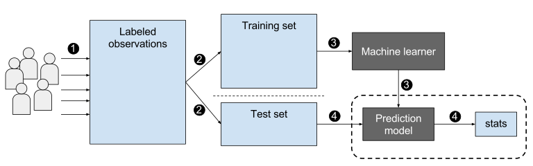
Features are the inputs that are given to the machine learning algorithm, the inputs that will be used to calculate an output value. In a mathematical sense, the features of the dataset are the variables used to solve the equation. The other part of the equation is the label or target, which are the classes the instances will be categorized into. Because the labels contain the target values for the machine learning classifier, when training a classifier you should split up the data into training and testing sets. The training set will have targets/labels, while the testing set won't contain these values.

Scikit-Learn, or "sklearn", is a machine learning library created for Python, intended to expedite machine learning tasks by making it easier to implement machine learning algorithms. It has easy-to-use functions to assist with splitting data into training and testing sets, as well as training a model, making predictions, and evaluating the model.

How Gradient Boosting Came to Be

The idea behind "gradient boosting" is to take a weak hypothesis or weak learning algorithm and make a series of tweaks to it that will improve the strength of the hypothesis/learner. This type of Hypothesis Boosting is based on the idea of Probability Approximately Correct Learning (PAC).

This PAC learning method investigates machine learning problems to interpret how complex they are, and a similar method is applied to Hypothesis Boosting.

In hypothesis boosting, you look at all the observations that the machine learning algorithm is trained on, and you leave only the observations that the machine learning method successfully classified behind, stripping out the other observations. A new weak learner is created and tested on the set of data that was poorly classified, and then just the examples that were successfully classified are kept.

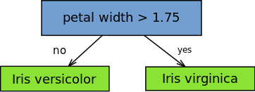
This idea was realized in the Adaptive Boosting (AdaBoost) algorithm. For AdaBoost, many weak learners are created by initializing many decision tree algorithms that only have a single split, such as the "stump" in the image below.

The instances/observations in the training set are weighted by the algorithm, and more weight is assigned to instances which are difficult to classify. More weak learners are added into the system sequentially, and they are assigned to the most difficult training instances.

In AdaBoost, the predictions are made through majority vote, with the instances being classified according to which class receives the most votes from the weak learners.

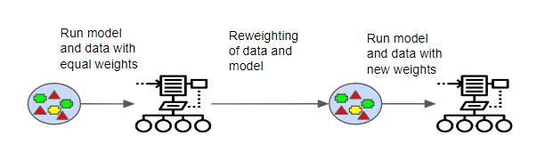
Gradient boosting classifiers are the AdaBoosting method combined with weighted minimization, after which the classifiers and weighted inputs are recalculated. The objective of Gradient Boosting classifiers is to minimize the loss, or the difference between the actual class value of the training example and the predicted class value. It isn't required to understand the process for reducing the classifier's loss, but it operates similarly to gradient descent in a neural network.

Refinements to this process were made and Gradient Boosting Machines were created.

In the case of Gradient Boosting Machines, every time a new weak learner is added to the model, the weights of the previous learners are frozen or cemented in place, left unchanged as the new layers are introduced. This is distinct from the approaches used in AdaBoosting where the values are adjusted when new learners are added.

The power of gradient boosting machines comes from the fact that they can be used on more than binary classification problems, they can be used on multi-class classification problems and even regression problems.

Theory Behind Gradient Boost

The Gradient Boosting Classifier depends on a loss function. A custom loss function can be used, and many standardized loss functions are supported by gradient boosting classifiers, but the loss function has to be differentiable.

Classification algorithms frequently use logarithmic loss, while regression algorithms can use squared errors. Gradient boosting systems don't have to derive a new loss function every time the boosting algorithm is added, rather any differentiable loss function can be applied to the system.

Gradient boosting systems have two other necessary parts: a weak learner and an additive component. Gradient boosting systems use decision trees as their weak learners. Regression trees are used for the weak learners, and these regression trees output real values. Because the outputs are real values, as new learners are added into the model the output of the regression trees can be added together to correct for errors in the predictions.

The additive component of a gradient boosting model comes from the fact that trees are added to the model over time, and when this occurs the existing trees aren't manipulated, their values remain fixed.

A procedure similar to gradient descent is used to minimize the error between given parameters. This is done by taking the calculated loss and performing gradient descent to reduce that loss. Afterwards, the parameters of the tree are modified to reduce the residual loss.

The new tree's output is then appended to the output of the previous trees used in the model. This process is repeated until a previously specified number of trees is reached, or the loss is reduced below a certain threshold.

Steps to Gradient Boosting

In order to implement a gradient boosting classifier, we'll need to carry out a number of different steps. We'll need to:

• Fit the model
• Tune the model's parameters and Hyperparameters
• Make predictions
• Interpret the results

Fitting models with Scikit-Learn is fairly easy, as we typically just have to call the fit() command after setting up the model.

However, tuning the model's hyperparameters requires some active decision making on our part. There are various arguments/hyperparameters we can tune to try and get the best accuracy for the model. One of the ways we can do this is by altering the learning rate of the model. We'll want to check the performance of the model on the training set at different learning rates, and then use the best learning rate to make predictions.

Predictions can be made in Scikit-Learn very simply by using the predict() function after fitting the classifier. You'll want to predict on the features of the testing dataset, and then compare the predictions to the actual labels. The process of evaluating a classifier typically involves checking the accuracy of the classifier and then tweaking the parameters/hyperparameters of the model until the classifier has an accuracy that the user is satisfied with.

Different Improved Gradient Boosting Classifiers

Because of the fact that grading boosting algorithms can easily overfit on a training data set, different constraints or regularization methods can be utilized to enhance the algorithm's performance and combat overfitting. Penalized learning, tree constraints, randomized sampling, and shrinkage can be utilized to combat overfitting.

Penalized Learning

Certain constraints can be utilized to prevent overfitting, depending on the structure of the decision tree. The type of decision tree used in gradient boosting is a regression tree, which has numeric values as leaves or weights. These weight values can be regularized using the different regularization methods, like L1 or L2 regularization weights, which penalizes the radiant boosting algorithm.

Tree Constraints

The decision tree can be constrained in numerous ways, such as limiting the tree depth, imposing a limit on the number of leaves or nodes of the tree, limiting the number of observations per split, and limiting the number of observations trained on. In general, the more constraints you use when creating trees, the more trees the model will need to properly fit the data.

Random Sampling/Stochastic Boosting

Taking random subsamples of the training data set, a technique referred to as stochastic gradient boosting, can also help prevent overfitting. This technique essentially reduces the strength of the correlation between trees.

There are multiple ways to subsample the data set, such as subsampling columns before each split, subsampling columns before creating a tree, as subsampling rows before creating a tree. In general, subsampling at large rates not exceeding 50% of the data seems to be beneficial to the model.

Shrinkage/Weighted Updates

Because the predictions of each tree are summed together, the contributions of the trees can be inhibited or slowed down using a technique called shrinkage. A "learning rate" is adjusted, and when the learning rate is reduced more trees must be added to the model. This makes it so that the model needs longer to train.

There's a trade-off between the learning rate and the number of trees needed, so you'll have to experiment to find the best values for each of the parameters, but small values less than 0.1 or values between 0.1 and 0.3 often work well.

XGBoost

XGBoost is a refined and customized version of a gradient boosting decision tree system, created with performance and speed in mind. XGBoost actually stands for "eXtreme Gradient Boosting", and it refers to the fact that the algorithms and methods have been customized to push the limit of what is possible for gradient boosting algorithms.

We'll be comparing a regular boosting classifier and an XGBoost classifier in the following section.

Implementing A Gradient Boosting Classifier

We'll now go over the implementation of a simple gradient boosting classifier and an XGBoost classifier. We'll begin with the simple boosting classifier.

Regular Boosting Classifier

To start with, we need to choose a dataset to work on, and for this example we'll be using the Titanic Dataset. You can download the data here.

Let's start by importing all our libraries:

import pandas as pd
from sklearn.preprocessing import MinMaxScaler
from sklearn.model_selection import train_test_split
from sklearn.metrics import classification_report, confusion_matrix
from sklearn.ensemble import GradientBoostingClassifier

Now let's load in our training data:

train_data = pd.read_csv("train.csv")
test_data = pd.read_csv("test.csv")

We may need to do some preprocessing of the data. Let's set the index as the PassengerId and then select our features and labels. Our label data, the y data is the Survived column. So we'll make that it's own dataframe and then remove it from the features:

y_train = train_data["Survived"]
train_data.drop(labels="Survived", axis=1, inplace=True)

Now we have to create a concatenated new data set:

full_data = train_data.append(test_data)

Let's drop any columns that aren't necessary or helpful for training, although you could leave them in and see how they affect things:

drop_columns = ["Name", "Age", "SibSp", "Ticket", "Cabin", "Parch", "Embarked"]
full_data.drop(labels=drop_columns, axis=1, inplace=True)

Any text data needs to be converted into numbers that our model can use, so let's change that now. We'll also fill any empty cells with 0:

full_data = pd.get_dummies(full_data, columns=["Sex"])
full_data.fillna(value=0.0, inplace=True)

Let's split the data into training and testing sets:

X_train = full_data.values[0:891]
X_test = full_data.values[891:]

We'll now scale our data by creating an instance of the scaler and scaling it:

scaler = MinMaxScaler()
X_train = scaler.fit_transform(X_train)
X_test = scaler.transform(X_test)

Now we can split the data into training and testing sets. Let's also set a seed (so you can replicate the results) and select the percentage of the data for testing on:

state = 12  
test_size = 0.30  
  
X_train, X_val, y_train, y_val = train_test_split(X_train, y_train,  
    test_size=test_size, random_state=state)

Now we can try setting different learning rates, so that we can compare the performance of the classifier's performance at different learning rates.

lr_list = [0.05, 0.075, 0.1, 0.25, 0.5, 0.75, 1]

for learning_rate in lr_list:
    gb_clf = GradientBoostingClassifier(n_estimators=20, learning_rate=learning_rate, max_features=2, max_depth=2, random_state=0)
    gb_clf.fit(X_train, y_train)

    print("Learning rate: ", learning_rate)
    print("Accuracy score (training): {0:.3f}".format(gb_clf.score(X_train, y_train)))
    print("Accuracy score (validation): {0:.3f}".format(gb_clf.score(X_val, y_val)))

Let's see what the performance was for different learning rates:

Learning rate:  0.05
Accuracy score (training): 0.801
Accuracy score (validation): 0.731

Learning rate:  0.075
Accuracy score (training): 0.814
Accuracy score (validation): 0.731

Learning rate:  0.1
Accuracy score (training): 0.812
Accuracy score (validation): 0.724

Learning rate:  0.25
Accuracy score (training): 0.835
Accuracy score (validation): 0.750

Learning rate:  0.5
Accuracy score (training): 0.864
Accuracy score (validation): 0.772

Learning rate:  0.75
Accuracy score (training): 0.875
Accuracy score (validation): 0.754

Learning rate:  1
Accuracy score (training): 0.875
Accuracy score (validation): 0.739

We're mainly interested in the classifier's accuracy on the validation set, but it looks like a learning rate of 0.5 gives us the best performance on the validation set and good performance on the training set.

Now we can evaluate the classifier by checking its accuracy and creating a confusion matrix. Let's create a new classifier and specify the best learning rate we discovered.

gb_clf2 = GradientBoostingClassifier(n_estimators=20, learning_rate=0.5, max_features=2, max_depth=2, random_state=0)
gb_clf2.fit(X_train, y_train)
predictions = gb_clf2.predict(X_val)

print("Confusion Matrix:")
print(confusion_matrix(y_val, predictions))

print("Classification Report")
print(classification_report(y_val, predictions))

Here's the output of our tuned classifier:

Confusion Matrix:
[[142  19]
 [ 42  65]]
Classification Report
              precision    recall  f1-score   support

           0       0.77      0.88      0.82       161
           1       0.77      0.61      0.68       107

    accuracy                           0.77       268
   macro avg       0.77      0.74      0.75       268
weighted avg       0.77      0.77      0.77       268

XGBoost Classifier

Now we'll experiment with the XGBoost classifier.

As before, let's start by importing the libraries we need.

from xgboost import XGBClassifier

Since our data is already prepared, we just need to fit the classifier with the training data:

xgb_clf = XGBClassifier()
xgb_clf.fit(X_train, y_train)

Now that the classifier has been fit and trained, we can check the score it achieves on the validation set by using the score command.

score = xgb_clf.score(X_val, y_val)
print(score)

Here's the output:

0.7761194029850746

Alternatively, you could predict the X_val data and then check the accuracy against the y_val by using accuracy_score. It should give you the same kind of result.

Comparing the accuracy of XGboost to the accuracy of a regular gradient classifier shows that, in this case, the results were very similar. However, this won't always be the case and in different circumstances, one of the classifiers could easily perform better than the other. Try varying the arguments in this model to see how the result differ.

Conclusion

Gradient boosting models are powerful algorithms which can be used for both classification and regression tasks. Gradient boosting models can perform incredibly well on very complex datasets, but they are also prone to overfitting, which can be combated with several of the methods described above. Gradient boosting classifiers are also easy to implement in Scikit-Learn.

Now that we've implemented both a regular boosting classifier and an XGBoost classifier, try implementing them both on the same dataset and see how the performance of the two classifiers compares.

If you'd like to learn more about the theory behind Gradient Boosting, you can read more about that here. You may also want to know more about the other classifiers that Scikit-Learn supports, so you can compare their performance. Learn more about Scikit-Learn's classifiers here.

If you'd like to play around with the code, it's up on GitHub!