
Introduction
This tutorial is an introduction to a simple optimization technique called gradient descent, which has seen major application in state-of-the-art machine learning models.
We'll develop a general purpose routine to implement gradient descent and apply it to solve different problems, including classification via supervised learning.
In this process, we'll gain an insight into the working of this algorithm and study the effect of various hyper-parameters on its performance. We'll also go over batch and stochastic gradient descent variants as examples.
What is Gradient Descent?
Gradient descent is an optimization technique that can find the minimum of an objective function. It is a greedy technique that finds the optimal solution by taking a step in the direction of the maximum rate of decrease of the function.
By contrast, Gradient Ascent is a close counterpart that finds the maximum of a function by following the direction of the maximum rate of increase of the function.
To understand how gradient descent works, consider a multivariable function \(f(\textbf{w})\), where \(\textbf w = [w_1, w_2, \ldots, w_n]^T \). To find the \( \textbf{w} \) at which this function attains a minimum, gradient descent uses the following steps:
-
Choose an initial random value of \( \textbf{w} \)
-
Choose the number of maximum iterations
T -
Choose a value for the learning rate \( \eta \in [a,b] \)
-
Repeat following two steps until \(f\) does not change or iterations exceed T
a.Compute: \( \Delta \textbf{w} = - \eta \nabla_\textbf{w} f(\textbf{w}) \)
b. update \(\textbf{w} \) as: \(\textbf{w} \leftarrow \textbf{w} + \Delta \textbf{w} \)
The left arrow symbol being a mathematically correct way to write an assignment statement.
Here \( \nabla_\textbf{w} f \) denotes the gradient of \(f\) as given by:
$$
\nabla_\textbf{w} f(\textbf{w}) =
\begin{bmatrix}
\frac{\partial f(\textbf{w})}{\partial w_1} \
\frac{\partial f(\textbf{w})}{\partial w_2} \
\vdots\
\frac{\partial f(\textbf{w})}{\partial w_n}
\end{bmatrix}
$$
Consider an example function of two variables \( f(w_1,w_2) = w_1^2+w_2^2 \), then at each iteration \( (w_1,w_2) \) is updated as:
$$
\begin {bmatrix}
w_1 \ w_2
\end {bmatrix} \leftarrow
\begin {bmatrix}
w_1 \ w_2
\end {bmatrix} - \eta
\begin {bmatrix}
2w_1 \ 2w_2
\end {bmatrix}
$$
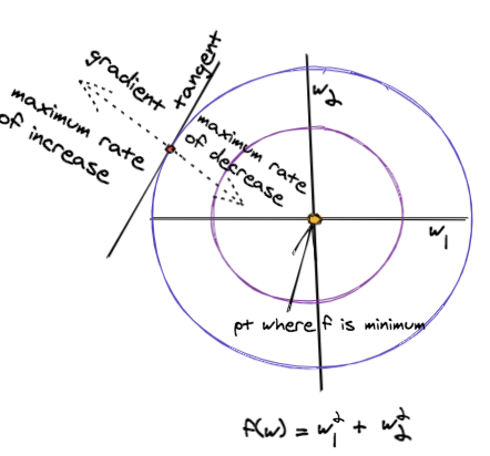
The figure below shows how gradient descent works on this function.
The circles are the contours of this function. If we move along a contour, the function value would not change and would remain a constant.
This is opposed to the direction of the gradient, where the function changes at a maximum rate. Therefore the direction of the gradient of the function at any point is normal to the contour's tangent at that point.
In simple terms, the gradient can be taken as an arrow which points in the direction where the function changes the most.
Following the negative gradient direction would lead to points where the function value decreases at a maximum rate. The learning rate, also called the step size, dictates how fast or slow, we move along the direction of the gradient.
Adding Momentum
When using gradient descent, we run into the following problems:
-
Getting trapped in a local minimum, which is a direct consequence of this algorithm being greedy
-
Overshooting and missing the global optimum, this is a direct result of moving too fast along the gradient direction
-
Oscillation, this is a phenomenon that occurs when the function's value doesn't change significantly no matter the direction it advances. You can think of it as navigating a plateau, you're at the same height no matter where you go
To combat these problems, a momentum term \( \alpha \) is added to the expression for \(\Delta \textbf{w}\) to stabilize the rate of learning when moving towards the global optimum value.
Below, we use the superscript \(i\) to denote the iteration number:
$$
\Delta \textbf{w}^i = - \eta \nabla_\textbf{w} f(\textbf{w}^i) + \alpha \textbf{w}^{i-1}
$$
Implementing Gradient Descent in Python
Before we start writing the actual code for gradient descent, let's import some libraries we'll utilize to help us out:
import numpy as np
import matplotlib
import matplotlib.pyplot as plt
import sklearn.datasets as dt
from sklearn.model_selection import train_test_split
Now, with that out of the way, let's go ahead and define a gradient_descent() function. In this function, the loop ends when either:
-
The number of iterations exceeds a maximum value
-
The difference in function values between two successive iterations falls below a certain threshold
The parameters are updated at every iteration according to the gradient of the objective function.
The function will accept the following parameters:
-
max_iterations: Maximum number of iterations to run -
threshold: Stop if the difference in function values between two successive iterations falls below this threshold -
w_init: Initial point from where to start gradient descent -
obj_func: Reference to the function that computes the objective function -
grad_func: Reference to the function that computes the gradient of the function -
extra_param: Extra parameters (if needed) for the obj_func and grad_func -
learning_rate: Step size for gradient descent. It should be in [0,1] -
momentum: Momentum to use. It should be in [0,1]
Also, the function will return:
-
w_history: All points in space, visited by gradient descent at which the objective function was evaluated -
f_history: Corresponding value of the objective function computed at each point
# Make threshold a -ve value if you want to run exactly
# max_iterations.
def gradient_descent(max_iterations,threshold,w_init,
                     obj_func,grad_func,extra_param = [],
                     learning_rate=0.05,momentum=0.8):

    w = w_init
    w_history = w
    f_history = obj_func(w,extra_param)
    delta_w = np.zeros(w.shape)
    i = 0
    diff = 1.0e10

    while  i<max_iterations and diff>threshold:
        delta_w = -learning_rate*grad_func(w,extra_param) + momentum*delta_w
        w = w+delta_w

        # store the history of w and f
        w_history = np.vstack((w_history,w))
        f_history = np.vstack((f_history,obj_func(w,extra_param)))

        # update iteration number and diff between successive values
        # of objective function
        i+=1
        diff = np.absolute(f_history[-1]-f_history[-2])

    return w_history,f_history
Optimizing Functions with Gradient Descent
Now that we have a general purpose implementation of gradient descent, let's run it on our example 2D function \( f(w_1,w_2) = w_1^2+w_2^2 \) with circular contours.
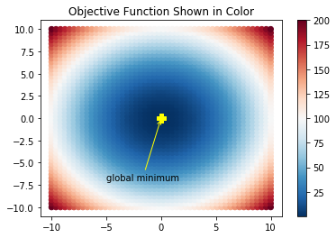
The function has a minimum value of zero at the origin. Let's visualize the function first and then find its minimum value.
Visualizing the Objective Function f(x)
The visualize_fw() function below, generates 2500 equally spaced points on a grid and computes the function value at each point.
The function_plot() function displays all points in different colors, depending upon the value of \(f(\textbf w)\) at that point. All points at which the function's value is the same, have the same color:
def visualize_fw():
    xcoord = np.linspace(-10.0,10.0,50)
    ycoord = np.linspace(-10.0,10.0,50)
    w1,w2 = np.meshgrid(xcoord,ycoord)
    pts = np.vstack((w1.flatten(),w2.flatten()))

    # All 2D points on the grid
    pts = pts.transpose()

    # Function value at each point
    f_vals = np.sum(pts*pts,axis=1)
    function_plot(pts,f_vals)
    plt.title('Objective Function Shown in Color')
    plt.show()
    return pts,f_vals

# Helper function to annotate a single point
def annotate_pt(text,xy,xytext,color):
    plt.plot(xy[0],xy[1],marker='P',markersize=10,c=color)
    plt.annotate(text,xy=xy,xytext=xytext,
                 # color=color,
                 arrowprops=dict(arrowstyle="->",
                 color = color,
                 connectionstyle='arc3'))

# Plot the function
# Pts are 2D points and f_val is the corresponding function value
def function_plot(pts,f_val):
    f_plot = plt.scatter(pts[:,0],pts[:,1],
                         c=f_val,vmin=min(f_val),vmax=max(f_val),
                         cmap='RdBu_r')
    plt.colorbar(f_plot)
    # Show the optimal point
    annotate_pt('global minimum',(0,0),(-5,-7),'yellow')

pts,f_vals = visualize_fw()
Running Gradient Descent with Different Hyper-parameters
Now it's time to run gradient descent to minimize our objective function. To call gradient_descent(), we define two functions:
f(): Computes the objective function at any pointwgrad(): Computes the gradient at any pointw
To understand the effect of various hyper-parameters on gradient descent, the function solve_fw() calls gradient_descent() with 5 iterations for different values of learning rate and momentum.
The function visualize_learning(), plots the values of \((w_1,w_2) \), with function values shown in different colors. The arrows in the plot make it easier to track which point was updated from the last:
# Objective function
def f(w,extra=[]):
    return np.sum(w*w)

# Function to compute the gradient
def grad(w,extra=[]):
    return 2*w

# Function to plot the objective function
# and learning history annotated by arrows
# to show how learning proceeded
def visualize_learning(w_history):

    # Make the function plot
    function_plot(pts,f_vals)

    # Plot the history
    plt.plot(w_history[:,0],w_history[:,1],marker='o',c='magenta')

    # Annotate the point found at last iteration
    annotate_pt('minimum found',
                (w_history[-1,0],w_history[-1,1]),
                (-1,7),'green')
    iter = w_history.shape[0]
    for w,i in zip(w_history,range(iter-1)):
        # Annotate with arrows to show history
        plt.annotate("",
                    xy=w, xycoords='data',
                    xytext=w_history[i+1,:], textcoords='data',
                    arrowprops=dict(arrowstyle='<-',
                            connectionstyle='angle3'))

def solve_fw():
    # Setting up
    rand = np.random.RandomState(19)
    w_init = rand.uniform(-10,10,2)
    fig, ax = plt.subplots(nrows=4, ncols=4, figsize=(18, 12))
    learning_rates = [0.05,0.2,0.5,0.8]
    momentum = [0,0.5,0.9]
    ind = 1

    # Iteration through all possible parameter combinations
    for alpha in momentum:
        for eta,col in zip(learning_rates,[0,1,2,3]):
            plt.subplot(3,4,ind)
            w_history,f_history = gradient_descent(5,-1,w_init, f,grad,[],eta,alpha)

            visualize_learning(w_history)
            ind = ind+1
            plt.text(-9, 12,'Learning Rate = '+str(eta),fontsize=13)
            if col==1:
                plt.text(10,15,'momentum = ' + str(alpha),fontsize=20)

    fig.subplots_adjust(hspace=0.5, wspace=.3)
    plt.show()
Let's run solve_fw() and see how the learning rate and momentum effect gradient descent:
solve_fw()
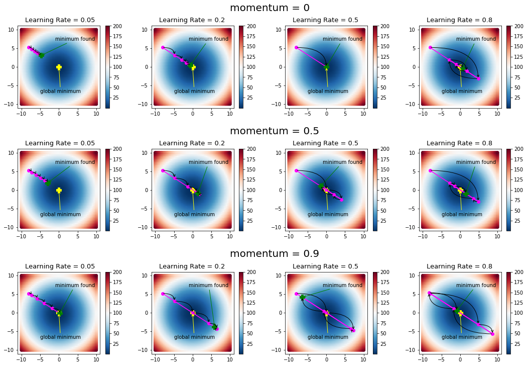
This example clarifies the role of both momentum and learning rate.
In the first plot, with zero momentum and learning rate set at 0.05, learning is slow and the algorithm does not reach the global minimum. Increasing the momentum speeds up learning as we can see from the plots in the first column. The other extreme is the last column, where the learning rate is kept high. This causes oscillations, which can be controlled to a certain extent by adding momentum.
Check out our hands-on, practical guide to learning Git, with best-practices, industry-accepted standards, and included cheat sheet. Stop Googling Git commands and actually learn it!
The general guideline for gradient descent is to use small values of learning rate and higher values of momentum.
Gradient Descent for Minimizing Mean Square Error
Gradient descent is a nice and simple technique for minimizing the mean square error in a supervised classification or regression problem.
Suppose we are given \(m\) training examples \([x_{ij}]\) with \(i=1\ldots m \), where each example has \(n\) features, i.e., \(j=1\ldots n \). If the corresponding target and output values for each example are \(t_i\) and \(o_i\) respectively, then the mean square error function \(E\) (in this case our object function) is defined as:
$$
E = \frac{1}{m} \Sigma_{i=1}^m (t_i - o_i)^2
$$
Where the output \(o_i\) is determined by a weighted linear combination of inputs, given by:
$$
o_i = w_0 + w_1 x_{i1} + w_2 x_{i2} + \ldots + w_n x_{in}
$$
The unknown parameter in the above equation is the weight vector \(\textbf w = [w_0,w_1,\ldots,w_n]^T\).
The objective function in this case is the mean square error with a gradient given by:
$$
\nabla_{\textbf w}E(\textbf w) = -\Sigma_{i=1}^{m} (t_i - o_i) \textbf{x}_i
$$
Where \(x_{i}\) is the i-th example. or an array of features of size n.
All we need now is a function to compute the gradient and a function to compute the mean square error.
The gradient_descent() function can then be used as-is. Note that all training examples are processed together when computing the gradient. Hence, this version of gradient descent for updating weights is referred to as batch updating or batch learning:
# Input argument is weight and a tuple (train_data, target)
def grad_mse(w,xy):
    (x,y) = xy
    (rows,cols) = x.shape

    # Compute the output
    o = np.sum(x*w,axis=1)
    diff = y-o
    diff = diff.reshape((rows,1))
    diff = np.tile(diff, (1, cols))
    grad = diff*x
    grad = -np.sum(grad,axis=0)
    return grad

# Input argument is weight and a tuple (train_data, target)
def mse(w,xy):
    (x,y) = xy

    # Compute output
    # keep in mind that we're using mse and not mse/m
    # because it would be relevant to the end result
    o = np.sum(x*w,axis=1)
    mse = np.sum((y-o)*(y-o))
    mse = mse/2
    return mse
Running Gradient Descent on OCR
To illustrate gradient descent on a classification problem, we have chosen the digits datasets included in sklearn.datasets.
To keep things simple, let's do a test run of gradient descent on a two-class problem (digit 0 vs. digit 1). The code below loads the digits and displays the first 10 digits. This gives us an idea of the nature of training points:
# Load the digits dataset with two classes
digits,target = dt.load_digits(n_class=2,return_X_y=True)
fig,ax = plt.subplots(nrows=1, ncols=10,figsize=(12,4),subplot_kw=dict(xticks=[], yticks=[]))

# Plot some images of digits
for i in np.arange(10):
    ax[i].imshow(digits[i,:].reshape(8,8),cmap=plt.cm.gray)
plt.show()

We also need the method train_test_split from sklearn.model_selection to split the training data into a train and a test set. The code below runs gradient descent on the training set, learns the weights, and plots the mean square error at different iterations.
When running gradient descent, we'll keep learning rate and momentum very small as the inputs are not normalized or standardized. Also, the batch version of gradient descent requires a smaller learning rate:
# Split into train and test set
x_train, x_test, y_train, y_test = train_test_split(
                        digits, target, test_size=0.2, random_state=10)

# Add a column of ones to account for bias in train and test
x_train = np.hstack((np.ones((y_train.size,1)),x_train))
x_test  = np.hstack((np.ones((y_test.size,1)),x_test))

# Initialize the weights and call gradient descent
rand = np.random.RandomState(19)
w_init = rand.uniform(-1,1,x_train.shape[1])*.000001
w_history,mse_history = gradient_descent(100,0.1,w_init,
                              mse,grad_mse,(x_train,y_train),
                             learning_rate=1e-6,momentum=0.7)

# Plot the MSE
plt.plot(np.arange(mse_history.size),mse_history)
plt.xlabel('Iteration No.')
plt.ylabel('Mean Square Error')
plt.title('Gradient Descent on Digits Data (Batch Version)')
plt.show()
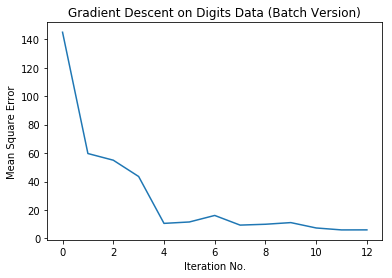
This looks great! Let's check the error rate of our OCR on the training and test data. Below is a small function to compute the error rate of classification, which is called on the training and test set:
# Returns error rate of classifier
# total misclassifications/total*100
def error(w,xy):
    (x,y) = xy
    o = np.sum(x*w,axis=1)

    #map the output values to 0/1 class labels
    ind_1 = np.where(o>0.5)
    ind_0 = np.where(o<=0.5)
    o[ind_1] = 1
    o[ind_0] = 0
    return np.sum((o-y)*(o-y))/y.size*100

train_error = error(w_history[-1],(x_train,y_train))
test_error = error(w_history[-1],(x_test,y_test))

print("Train Error Rate: " + "{:.2f}".format(train_error))
print("Test Error Rate: " + "{:.2f}".format(test_error))
Train Error Rate: 0.69
Test Error Rate: 1.39
Stochastic Gradient Descent in Python
In the previous section, we used the batch updating scheme for gradient descent.
Another version of gradient descent is the online or stochastic updating scheme, where each training example is taken one at a time for updating the weights.
Once all training examples are cycled through, we say that an epoch is completed. The training examples are shuffled before each epoch, for better results.
The code snippet below is a slight modification of the gradient_descent() function to incorporate its stochastic counterpart. This function takes the (training set, target) as a parameter instead of the extra parameter. The term 'iterations' has been renamed to 'epochs':
# (xy) is the (training_set,target) pair
def stochastic_gradient_descent(max_epochs,threshold,w_init,
                                obj_func,grad_func,xy,
                                learning_rate=0.05,momentum=0.8):
    (x_train,y_train) = xy
    w = w_init
    w_history = w
    f_history = obj_func(w,xy)
    delta_w = np.zeros(w.shape)
    i = 0
    diff = 1.0e10
    rows = x_train.shape[0]

    # Run epochs
    while  i<max_epochs and diff>threshold:
        # Shuffle rows using a fixed seed to reproduce the results
        np.random.seed(i)
        p = np.random.permutation(rows)

        # Run for each instance/example in training set
        for x,y in zip(x_train[p,:],y_train[p]):
            delta_w = -learning_rate*grad_func(w,(np.array([x]),y)) + momentum*delta_w
            w = w+delta_w

        i+=1
        w_history = np.vstack((w_history,w))
        f_history = np.vstack((f_history,obj_func(w,xy)))
        diff = np.absolute(f_history[-1]-f_history[-2])

    return w_history,f_history
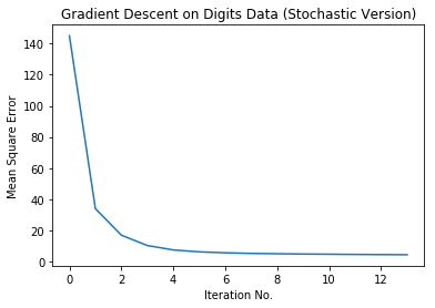
Let's run the code to see how the results are for stochastic version of gradient descent:
rand = np.random.RandomState(19)
w_init = rand.uniform(-1,1,x_train.shape[1])*.000001
w_history_stoch,mse_history_stoch = stochastic_gradient_descent(
                                100,0.1,w_init,
                              mse,grad_mse,(x_train,y_train),
                             learning_rate=1e-6,momentum=0.7)

# Plot the MSE
plt.plot(np.arange(mse_history_stoch.size),mse_history_stoch)
plt.xlabel('Iteration No.')
plt.ylabel('Mean Square Error')
plt.title('Gradient Descent on Digits Data (Stochastic Version)')

plt.show()
Let's also check the error rate:
train_error_stochastic = error(w_history_stoch[-1],(x_train,y_train))
test_error_stochastic = error(w_history_stoch[-1],(x_test,y_test))

print("Train Error rate with Stochastic Gradient Descent: " +
      "{:.2f}".format(train_error_stochastic))
print("Test Error rate with Stochastic Gradient Descent: "
      + "{:.2f}".format(test_error_stochastic))
Train Error rate with Stochastic Gradient Descent: 0.35
Test Error rate with Stochastic Gradient Descent: 1.39
Comparing Batch and Stochastic Versions
Let's now compare both the batch and stochastic versions of gradient descent.
We'll fix the learning rate for both versions to the same value and vary momentum to see how fast they both converge. The initial weights and the stopping criteria for both algorithms remain the same:
fig, ax = plt.subplots(nrows=3, ncols=1, figsize=(10,3))

rand = np.random.RandomState(11)
w_init = rand.uniform(-1,1,x_train.shape[1])*.000001
eta = 1e-6
for alpha,ind in zip([0,0.5,0.9],[1,2,3]):
    w_history,mse_history = gradient_descent(
                                100,0.01,w_init,
                              mse,grad_mse,(x_train,y_train),
                             learning_rate=eta,momentum=alpha)

    w_history_stoch,mse_history_stoch = stochastic_gradient_descent(
                                100,0.01,w_init,
                              mse,grad_mse,(x_train,y_train),
                             learning_rate=eta,momentum=alpha)

    # Plot the MSE
    plt.subplot(130+ind)
    plt.plot(np.arange(mse_history.size),mse_history,color='green')
    plt.plot(np.arange(mse_history_stoch.size),mse_history_stoch,color='blue')
    plt.legend(['batch','stochastic'])

    # Display total iterations
    plt.text(3,-30,'Batch: Iterations='+
             str(mse_history.size) )
    plt.text(3,-45,'Stochastic: Iterations='+
             str(mse_history_stoch.size))
    plt.title('Momentum = ' + str(alpha))

    # Display the error rates
    train_error = error(w_history[-1],(x_train,y_train))
    test_error = error(w_history[-1],(x_test,y_test))

    train_error_stochastic = error(w_history_stoch[-1],(x_train,y_train))
    test_error_stochastic = error(w_history_stoch[-1],(x_test,y_test))

    print ('Momentum = '+str(alpha))

    print ('\tBatch:')
    print ('\t\tTrain error: ' + "{:.2f}".format(train_error) )
    print ('\t\tTest error: ' + "{:.2f}".format(test_error) )

    print ('\tStochastic:')
    print ('\t\tTrain error: ' + "{:.2f}".format(train_error_stochastic) )
    print ('\t\tTest error: ' + "{:.2f}".format(test_error_stochastic) )


plt.show()
Momentum = 0
    Batch:
        Train error: 0.35
        Test error: 1.39
    Stochastic:
        Train error: 0.35
        Test error: 1.39
Momentum = 0.5
    Batch:
        Train error: 0.00
        Test error: 1.39
    Stochastic:
        Train error: 0.35
        Test error: 1.39
Momentum = 0.9
    Batch:
        Train error: 0.00
        Test error: 1.39
    Stochastic:
        Train error: 0.00
        Test error: 1.39
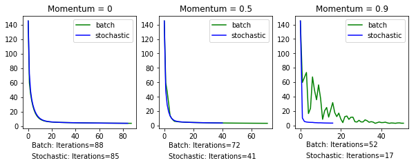
While there isn't a significant difference in the accuracy between the two versions of the classifier, the stochastic version is a clear winner when it comes to the speed of convergence. It takes fewer iterations to achieve the same result as its batch counterpart.
Conclusions
Gradient descent is a simple and easy to implement technique.
In this tutorial, we illustrated gradient descent on a function of two variables with circular contours. We then extended our example to minimize the mean square error in a classification problem and built a simple OCR system. We also discussed the stochastic version of gradient descent.
A general purpose function for implementing gradient descent was developed in this tutorial. We encourage the readers to use this function on different regression and classification problems, with different hyper-parameters, for a better understanding of its working.

