Image Recognition and Classification in Python with TensorFlow and Keras

Introduction

TensorFlowis a well-established Deep Learning framework, and Keras is its official high-level API that simplifies the creation of models. Image recognition/classification is a common task, and thankfully, it's fairly straightforward and simple with Keras.

In this guide, we'll take a look at how to classify/recognize images in Python with Keras.

In this guide, we'll be building a custom CNN and training it from scratch. For a more advanced guide, you can leverage Transfer Learning to transfer knowledge representations with existing highly-performant architectures - read our Image Classification with Transfer Learning in Keras - Create Cutting Edge CNN Models!

Definitions

If you aren't clear on the basic concepts behind image classification, it will be difficult to completely understand the rest of this guide. So before we proceed any further, let's take a moment to define some terms.

TensorFlow/Keras

TensorFlow is an open source library created for Python by the Google Brain team. TensorFlow compiles many different algorithms and models together, enabling the user to implement deep neural networks for use in tasks like image recognition/classification and natural language processing. TensorFlow is a powerful framework that functions by implementing a series of processing nodes, each node representing a mathematical operation, with the entire series of nodes being called a "graph".

In terms of Keras, it is a high-level API (application programming interface) that can use TensorFlow's functions underneath (as well as other ML libraries like Theano). Keras was designed with user-friendliness and modularity as its guiding principles. In practical terms, Keras makes implementing the many powerful but often complex functions of TensorFlow as simple as possible, and it's configured to work with Python without any major modifications or configuration.

Image Classification (Recognition)

Image recognition refers to the task of inputting an image into a neural network and having it output some kind of label for that image. The label that the network outputs will correspond to a predefined class. There can be multiple classes that the image can be labeled as, or just one. If there is a single class, the term "recognition" is often applied, whereas a multi-class recognition task is often called "classification".

A subset of image classification is object detection, where specific instances of objects are identified as belonging to a certain class like animals, cars, or people.

Feature Extraction

In order to carry out image recognition/classification, the neural network must carry out feature extraction. Features are the elements of the data that you care about which will be fed through the network. In the specific case of image recognition, the features are the groups of pixels, like edges and points, of an object that the network will analyze for patterns.

Feature recognition (or feature extraction) is the process of pulling the relevant features out from an input image so that these features can be analyzed. Many images contain annotations or metadata about the image that helps the network find the relevant features.

How Neural Networks Learn to Recognize Images - Primer on Convolutional Neural Networks

Getting an intuition of how a neural network recognizes images will help you when you are implementing a neural network model, so let's briefly explore the image recognition process in the next few sections.

This section is meant to serve as a crash course/primer on Convolutional Neural Networks, as well as a refresher for those familiar with them.

Feature Extraction With Filters

Credit: commons.wikimedia.org

The first layer of a neural network takes in all the pixels within an image. After all the data has been fed into the network, different filters are applied to the image, which forms representations of different parts of the image. This is feature extraction and it creates "feature maps".

This process of extracting features from an image is accomplished with a "convolutional layer", and convolution is simply forming a representation of part of an image. It is from this convolution concept that we get the term Convolutional Neural Network (CNN), the type of neural network most commonly used in image classification/recognition. Recently, Transformers have performed wonders in image classification as well, which are based on the Recurrent Neural Network (RNN) architecture.

If you want to visualize how creating feature maps for Convolutional Networks works - think about shining a flashlight over a picture in a dark room. As you slide the beam over the picture you are learning about features of the image. A filter is what the network uses to form a representation of the image, and in this metaphor, the light from the flashlight is the filter.

The width of your flashlight's beam controls how much of the image you examine at one time, and neural networks have a similar parameter, the filter size. Filter size affects how much of the image, how many pixels, are being examined at one time. A common filter size used in CNNs is 3, and this covers both height and width, so the filter examines a 3 x 3 area of pixels.

Credit: commons.wikimedia.org

While the filter size covers the height and width of the filter, the filter's depth must also be specified.

How does a 2D image have depth?

Digital images are rendered as height, width, and some RGB value that defines the pixel's colors, so the "depth" that is being tracked is the number of color channels the image has. Grayscale (non-color) images only have 1 color channel while color images have 3 depth channels.

All of this means that for a filter of size 3 applied to a full-color image, the dimensions of that filter will be 3 x 3 x 3. For every pixel covered by that filter, the network multiplies the filter values with the values in the pixels themselves to get a numerical representation of that pixel. This process is then done for the entire image to achieve a complete representation. The filter is moved across the rest of the image according to a parameter called "stride", which defines how many pixels the filter is to be moved by after it calculates the value in its current position. A conventional stride size for a CNN is 2.

The end result of all this calculation is a feature map. This process is typically done with more than one filter, which helps preserve the complexity of the image.

Activation Functions

After the feature map of the image has been created, the values that represent the image are passed through an activation function or activation layer. The activation function takes values that represent the image, which are in a linear form (i.e. just a list of numbers) thanks to the convolutional layer, and increases their non-linearity since images themselves are non-linear.

The typical activation function used to accomplish this is a Rectified Linear Unit (ReLU), although there are some other activation functions that are occasionally used (you can read about those here).

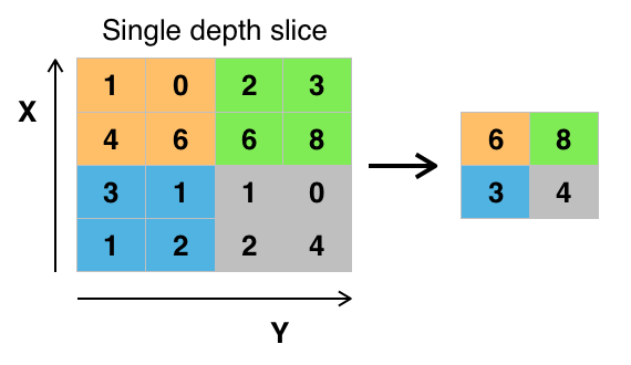
Pooling Layers

After the data is activated, it is sent through a pooling layer. Pooling "down-samples" an image, meaning that it takes the information which represents the image and compresses it, making it smaller. The pooling process makes the network more flexible and more adept at recognizing objects/images based on the relevant features.

When we look at an image, we typically aren't concerned with all the information in the background of the image, only the features we care about, such as people or animals.

Similarly, a pooling layer in CNN will abstract away the unnecessary parts of the image, keeping only the parts of the image it thinks are relevant, as controlled by the specified size of the pooling layer.

Because it has to make decisions about the most relevant parts of the image, the hope is that the network will learn only the parts of the image that truly represent the object in question. This helps prevent overfitting, where the network learns aspects of the training case too well and fails to generalize to new data.

Credit: commons.wikimedia.org

There are various ways to pool values, but max pooling is most commonly used. Max pooling obtains the maximum value of the pixels within a single filter (within a single spot in the image). This drops 3/4ths of information, assuming 2 x 2 filters are being used.

The maximum values of the pixels are used in order to account for possible image distortions, and the parameters/size of the image are reduced in order to control for overfitting. There are other pooling types such as average pooling or sum pooling, but these aren't used as frequently because max pooling tends to yield better accuracy.

Flattening

The final layers of our CNN, the densely connected layers, require that the data is in the form of a vector to be processed. For this reason, the data must be "flattened". The values are compressed into a long vector or a column of sequentially ordered numbers.

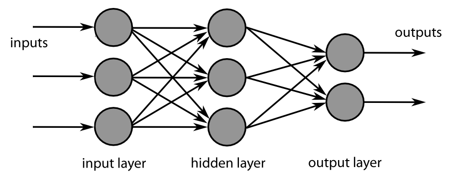
Fully Connected Layer

The final layers of the CNN are densely connected layers, or an artificial neural network (ANN). The primary function of the ANN is to analyze the input features and combine them into different attributes that will assist in classification. These layers are essentially forming collections of neurons that represent different parts of the object in question, and a collection of neurons may represent the floppy ears of a dog or the redness of an apple. When enough of these neurons are activated in response to an input image, the image will be classified as an object.

Credit: commons.wikimedia.org

The error, or the difference between the computed values and the expected value in the training set, is calculated by the ANN. The network then undergoes backpropagation, where the influence of a given neuron on a neuron in the next layer is calculated and its influence adjusted. This is done to optimize the performance of the model. This process is then repeated over and over. This is how the network trains on data and learns associations between input features and output classes.

The neurons in the middle fully connected layers will output binary values relating to the possible classes. If you have four different classes (let's say a dog, a car, a house, and a person), the neuron will have a "1" value for the class it believes the image represents and a "0" value for the other classes.

The final fully connected layer will receive the output of the layer before it and deliver a probability for each of the classes, summing to one. If there is a 0.75 value in the "dog" category, it represents a 75% certainty that the image is a dog.

The image classifier has now been trained, and images can be passed into the CNN, which will now output a guess about the content of that image.

The Machine Learning Workflow

Before we jump into an example of training an image classifier, let's take a moment to understand the machine learning workflow or pipeline. The process for training a neural network model is fairly standard and can be broken down into four different phases.

Data Preparation

First, you will need to collect your data and put it in a form the network can train on. This involves collecting images and labeling them. Even if you have downloaded a data set someone else has prepared, there is likely to be preprocessing or preparation that you must do before you can use it for training. Data preparation is an art all on its own, involving dealing with things like missing values, corrupted data, data in the wrong format, incorrect labels, etc.

In this article, we will be using a preprocessed data set.

Creating the Model

Creating the neural network model involves making choices about various parameters and hyperparameters. You must make decisions about the number of layers to use in your model, what the input and output sizes of the layers will be, what kind of activation functions you will use, whether or not you will use dropout, etc.

Learning which parameters and hyperparameters to use will come with time (and a lot of studying), but right out of the gate there are some heuristics you can use to get you running and we'll cover some of these during the implementation example.

Training the Model

After you have created your model, you simply create an instance of the model and fit it with your training data. The biggest consideration when training a model is the amount of time the model takes to train. You can specify the length of training for a network by specifying the number of epochs to train over. The longer you train a model, the greater its performance will improve, but too many training epochs and you risk overfitting.

Choosing the number of epochs to train for is something you will get a feel for, and it is customary to save the weights of a network in between training sessions so that you need not start over once you have made some progress training the network.

Model Evaluation

There are multiple steps to evaluating the model. The first step in evaluating the model is comparing the model's performance against a validation dataset, a data set that the model hasn't been trained on. You will compare the model's performance against this validation set and analyze its performance through different metrics.

There are various metrics for determining the performance of a neural network model, but the most common metric is "accuracy", the amount of correctly classified images divided by the total number of images in your data set.

After you have seen the accuracy of the model's performance on a validation dataset, you will typically go back and train the network again using slightly tweaked parameters, because it's unlikely you will be satisfied with your network's performance the first time you train. You will keep tweaking the parameters of your network, retraining it, and measuring its performance until you are satisfied with the network's accuracy.

Finally, you will test the network's performance on a testing set. This testing set is another set of data your model has never seen before.

Perhaps you are wondering:

Why bother with the testing set? If you are getting an idea of your model's accuracy, isn't that the purpose of the validation set?

It's a good idea to keep a batch of data the network has never seen for testing because all the tweaking of the parameters you do, combined with the retesting on the validation set, could mean that your network has learned some idiosyncrasies of the validation set which will not generalize to out-of-sample data.

Therefore, the purpose of the testing set is to check for issues like overfitting and be more confident that your model is truly fit to perform in the real world.

Image Recognition/Classification with a CNN in Keras

We've covered a lot so far, and if all this information has been a bit overwhelming, seeing these concepts come together in a sample classifier trained on a data set should make these concepts more concrete. So let's look at a full example of image recognition with Keras, from loading the data to evaluation.

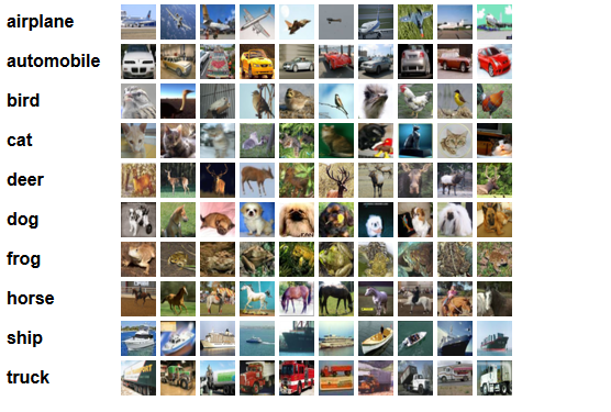
Credit: www.cs.toronto.edu

To begin with, we'll need a dataset to train on. In this example, we will be using the famous CIFAR-10 dataset. CIFAR-10 is a large image dataset containing over 60,000 images representing 10 different classes of objects like cats, planes, and cars.

The images are full-color RGB, but they are fairly small, only 32 x 32. One great thing about the CIFAR-10 dataset is that it comes prepackaged with Keras, so it is very easy to load up the dataset and the images need very little preprocessing.

The first thing we should do is import the necessary libraries. I'll show how these imports are used as we go, but for now know that we'll be making use of NumPy, and various modules associated with Keras:

import numpy
from tensorflow import keras
from keras.constraints import maxnorm
from keras.utils import np_utils

We're going to be using a random seed here so that the results achieved in this article can be replicated by you, which is why we need numpy:

# Set random seed for purposes of reproducibility
seed = 21

Prepping the Data

We need one more import: the dataset.

from keras.datasets import cifar10

Now let's load in the dataset. We can do so simply by specifying which variables we want to load the data into, and then using the load_data() function:

# Loading in the data
(X_train, y_train), (X_test, y_test) = cifar10.load_data()

In most cases you will need to do some preprocessing of your data to get it ready for use, but since we are using a prepackaged dataset, very little preprocessing needs to be done. One thing we want to do is normalize the input data.

If the values of the input data are in too wide a range it can negatively impact how the network performs. In this case, the input values are the pixels in the image, which have a value between 0 to 255.

So in order to normalize the data we can simply divide the image values by 255. To do this we first need to make the data a float type, since they are currently integers. We can do this by using the astype() NumPy command and then declaring what data type we want:

# Normalize the inputs from 0-255 to between 0 and 1 by dividing by 255
X_train = X_train.astype('float32')
X_test = X_test.astype('float32')
X_train = X_train / 255.0
X_test = X_test / 255.0

Another thing we'll need to do to get the data ready for the network is to one-hot encode the values. I won't go into the specifics of one-hot encoding here, but for now know that the images can't be used by the network as they are, they need to be encoded first and one-hot encoding is best used when doing binary classification.

We are effectively doing binary classification here because an image either belongs to one class or it doesn't, it can't fall somewhere in-between. The NumPy command to_categorical() is used to one-hot encode. This is why we imported the np_utils function from Keras, as it contains to_categorical().

We also need to specify the number of classes that are in the dataset, so we know how many neurons to compress the final layer down to:

# One-hot encode outputs
y_train = np_utils.to_categorical(y_train)
y_test = np_utils.to_categorical(y_test)
class_num = y_test.shape[1]

Designing the Model

We've reached the stage where we design the CNN model. The first thing to do is define the format we would like to use for the model. Keras has several different formats or blueprints to build models on, but Sequential is the most commonly used, and for that reason, we have imported it from Keras.

Create the Model

We can build the sequential model either by creating a blank instance and then adding layers to it:

model = Sequential()
model.add(keras.layers.layer1)
model.add(keras.layers.layer2)
model.add(keras.layers.layer3)

Or, we can pass in each layer as an element in a list in the Sequential() constructor call:

model = keras.Sequential([
    keras.layers.layer1,
    keras.layers.layer2,
    keras.layers.layer3    
])

The first layer of our model is a convolutional layer. It will take in the inputs and run convolutional filters on them.

When implementing these in Keras, we have to specify the number of channels/filters we want (that's the 32 below), the size of the filter we want (3 x 3 in this case), the input shape (when creating the first layer) and the activation and padding we need. These are all hyperparameters in the CNN which are prone to tuning. As mentioned, relu is the most common activation, and padding='same' just means we aren't changing the size of the image at all. You can try out other activation layers as well - though, relu is a very sensible default to first test out before tuning:

model = keras.Sequential()
model.add(keras.layers.Conv2D(32, (3, 3), input_shape=X_train.shape[1:], padding='same'))
model.add(keras.layers.Activation('relu'))

model.add(keras.layers.Conv2D(32, 3, input_shape=(32, 32, 3), activation='relu', padding='same'))

Now we will add a dropout layer to prevent overfitting, which functions by randomly eliminating some of the connections between the layers (0.2 means it drops 20% of the existing connections):

model.add(keras.layers.Dropout(0.2))

We may also want to add batch normalization here. Batch Normalization normalizes the inputs heading into the next layer, ensuring that the network always creates activations with the same distribution that we desire:

model.add(keras.layers.BatchNormalization())

This is the basic block used for building CNNs. Convolutional layer, activation, dropout, pooling. These blocks can then be stacked, typically in a pyramid pattern in terms of complexity. The next block typically contains a convolutional layer with a larger filter, which allows it to find patterns in greater detail and abstract further, followed by a pooling layer, dropout and batch normalization:

model.add(keras.layers.Conv2D(64, 3, activation='relu', padding='same'))
model.add(keras.layers.MaxPooling2D(2))
model.add(keras.layers.Dropout(0.2))
model.add(keras.layers.BatchNormalization())

You can vary the exact number of convolutional layers you have to your liking, though each one adds more computation expenses. Notice that as you add convolutional layers you typically increase their number of filters so the model can learn more complex representations. If the numbers chosen for these layers seem somewhat arbitrary, in general, you increase filters as you go on and it's advised to make them powers of 2 which can grant a slight benefit when training on a GPU.

It's important not to have too many pooling layers, as each pooling layer discards some data by slashing the dimensions of the input with a given factor. In our case, it cuts the images in half. Pooling too often will lead to there being almost nothing for the densely connected layers to learn about when the data reaches them.

The exact number of pooling layers you should use will vary depending on the task you are doing, and it's something you'll get a feel for over time. Since the images are so small here already we won't pool more than twice.

You can now repeat these layers to give your network more representations to work off of:

model.add(keras.layers.Conv2D(64, 3, activation='relu', padding='same'))
model.add(keras.layers.MaxPooling2D(2))
model.add(keras.layers.Dropout(0.2))
model.add(keras.layers.BatchNormalization())
    
model.add(keras.layers.Conv2D(128, 3, activation='relu', padding='same'))
model.add(keras.layers.Dropout(0.2))
model.add(keras.layers.BatchNormalization())

After we are done with the convolutional layers, we need to Flatten the data, which is why we imported the function above. We'll also add a layer of dropout again:

model.add(keras.layers.Flatten())
model.add(keras.layers.Dropout(0.2))

Now we make use of the Dense import and create the first densely connected layer. We need to specify the number of neurons in the dense layer. Note that the numbers of neurons in succeeding layers decreases, eventually approaching the same number of neurons as there are classes in the dataset (in this case 10).

We can have multiple dense layers here, and these layers extract information from the feature maps to learn to classify images based on the feature maps. Since we've got fairly small images condensed into fairly small feature maps - there's no need to have multiple dense layers. A single, simple, 32-neuron layer should be quite enough:

model.add(keras.layers.Dense(32, activation='relu'))
model.add(keras.layers.Dropout(0.3))
model.add(keras.layers.BatchNormalization())

In the final layer, we pass in the number of classes for the number of neurons. Each neuron represents a class, and the output of this layer will be a 10 neuron vector with each neuron storing some probability that the image in question belongs to the class it represents.

Finally, the softmax activation function selects the neuron with the highest probability as its output, voting that the image belongs to that class:

model.add(keras.layers.Dense(class_num, activation='softmax'))

Now that we've designed the model we want to use, we just have to compile it. The optimizer is what will tune the weights in your network to approach the point of lowest loss. The Adaptive Moment Estimation (Adam) algorithm is a very commonly used optimizer, and a very sensible default optimizer to try out. It's typically stable and performs well on a wide variety of tasks, so it'll likely perform well here.

If it doesn't, we can switch to a different optimizer, such as Nadam (Nesterov-accelerated Adam), RMSProp (oftentimes used for regression), etc.

We'll be keeping track of accuracy and validation accuracy to make sure we avoid overfitting CNN badly. If the two start diverging significantly and the network performs much better on the validation set - it's overfitting.

model.compile(loss='categorical_crossentropy', optimizer='adam', metrics=['accuracy', 'val_accuracy'])

We can print out the model summary to see what the whole model looks like.

print(model.summary())

Printing out the summary will give us quite a bit of info, and can be used to cross-check your own architecture against the one laid out in the guide:

_________________________________________________________________
Layer (type)                 Output Shape              Param #   
=================================================================
conv2d_43 (Conv2D)           (None, 32, 32, 32)        896       
_________________________________________________________________
dropout_50 (Dropout)         (None, 32, 32, 32)        0         
_________________________________________________________________
batch_normalization_44 (Batc (None, 32, 32, 32)        128       
_________________________________________________________________
conv2d_44 (Conv2D)           (None, 32, 32, 64)        18496     
_________________________________________________________________
max_pooling2d_20 (MaxPooling (None, 16, 16, 64)        0         
_________________________________________________________________
dropout_51 (Dropout)         (None, 16, 16, 64)        0         
_________________________________________________________________
batch_normalization_45 (Batc (None, 16, 16, 64)        256       
_________________________________________________________________
conv2d_45 (Conv2D)           (None, 16, 16, 64)        36928     
_________________________________________________________________
max_pooling2d_21 (MaxPooling (None, 8, 8, 64)          0         
_________________________________________________________________
dropout_52 (Dropout)         (None, 8, 8, 64)          0         
_________________________________________________________________
batch_normalization_46 (Batc (None, 8, 8, 64)          256       
_________________________________________________________________
conv2d_46 (Conv2D)           (None, 8, 8, 128)         73856     
_________________________________________________________________
dropout_53 (Dropout)         (None, 8, 8, 128)         0         
_________________________________________________________________
batch_normalization_47 (Batc (None, 8, 8, 128)         512       
_________________________________________________________________
flatten_6 (Flatten)          (None, 8192)              0         
_________________________________________________________________
dropout_54 (Dropout)         (None, 8192)              0         
_________________________________________________________________
dense_18 (Dense)             (None, 32)                262176    
_________________________________________________________________
dropout_55 (Dropout)         (None, 32)                0         
_________________________________________________________________
batch_normalization_48 (Batc (None, 32)                128       
_________________________________________________________________
dense_19 (Dense)             (None, 10)                330       
=================================================================
Total params: 393,962
Trainable params: 393,322
Non-trainable params: 640

Now we get to training the model. To do this, all we have to do is call the fit() function on the model and pass in the chosen parameters. We can additionally save its history as well, and plot its performance over the training process. This often gives us valuable information on the progress the network has made, and whether we could've trained it further and whether it'll start overfitting if we do so.

We've used a seed for reproducibility, so let's train the network and save its performance:

numpy.random.seed(seed)
history = model.fit(X_train, y_train, validation_data=(X_test, y_test), epochs=25, batch_size=64)

This results in:

Epoch 1/25
782/782 [==============================] - 12s 15ms/step - loss: 1.4851 - accuracy: 0.4721 - val_loss: 1.1805 - val_accuracy: 0.5777
...
Epoch 25/25
782/782 [==============================] - 11s 14ms/step - loss: 0.4154 - accuracy: 0.8538 - val_loss: 0.5284 - val_accuracy: 0.8197

Note that in most cases, you'd want to have a validation set that is different from the testing set, and so you'd specify a percentage of the training data to use as the validation set. In this case, we'll just pass in the test data to make sure the test data is set aside and not trained on. We'll only have test data in this example, in order to keep things simple.

Now we can evaluate the model and see how it performed. Just call model.evaluate():

# Model evaluation
scores = model.evaluate(X_test, y_test, verbose=0)
print("Accuracy: %.2f%%" % (scores[1]*100))

And we're greeted with the result:

Accuracy: 82.01%

With Transfer Learning and more powerful architectures, you can achieve much more. We showcase a 94% accuracy in our Guide to Image Classification with Transfer Learning in Keras - Create Cutting Edge CNN Models!

Additionally, we can visualize the history very easily:

import pandas as pd
import matplotlib.pyplot as plt

pd.DataFrame(history.history).plot()
plt.show()

This results in:

From the curves, we can see that the training hasn't actually halted after 25 epochs - it probably could've gone on for longer than that on this same model and architecture, which would've yielded a higher accuracy.

And that's it! We now have a trained image recognition CNN. Not bad for the first run, but you would probably want to play around with the model structure and parameters to see if you can't get better performance.

Conclusion

Now that you've implemented your first image recognition network in Keras, it would be a good idea to play around with the model and see how changing its parameters affects its performance.

This will give you some intuition about the best choices for different model parameters. You should also read up on the different parameter and hyper-parameter choices while you do so. After you are comfortable with these, you can try implementing your own image classifier on a different dataset.