Introduction to GANs with Python and TensorFlow

Introduction

Generative models are a family of AI architectures whose aim is to create data samples from scratch. They achieve this by capturing the data distributions of the type of things we want to generate.

These kinds of models are being heavily researched, and there is a huge amount of hype around them. Just look at the chart that shows the numbers of papers published in the field over the past few years:

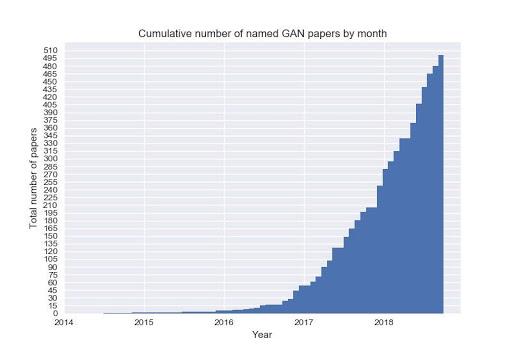
Since 2014, when the first paper on Generative Adversarial Networks was published, generative models are becoming incredibly powerful, and we are now able to generate hyper-realistic data samples for a wide range of distributions: images, videos, music, pieces of writing, etc.

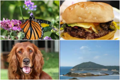
Here are some examples of images generated by a GAN:

What are Generative Models?

The GANs Framework

The most successful framework proposed for generative models, at least over recent years, takes the name of Generative Adversarial Networks (GANs).

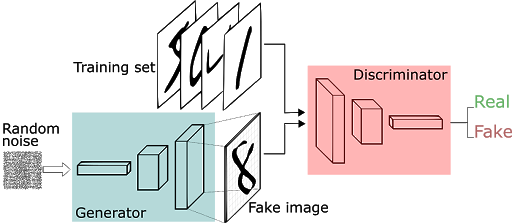
Simply put, a GAN is composed of two separate models, represented by neural networks: a generator G and a discriminator D. The goal of the discriminator is to tell whether a data sample comes from a real data distribution, or whether it is instead generated by G.

The goal of the generator is to generate data samples such as to fool the discriminator.

The generator is nothing but a deep neural network. It takes as input a vector of random noise (usually Gaussian or from a Uniform distribution) and outputs a data sample from the distribution we want to capture.

The discriminator is, again, just a neural network. Its goal is, as its name states, to discriminate between real and fake samples. Consequently, its input is a data sample, either coming from the generator or from the actual data distribution.

The output is a simple number, representing the probability that the input was real. A high probability means that the discriminator is confident that the samples he's being fed is a genuine one. On the contrary, a low probability shows high confidence in the fact that the sample is coming from the generator network:

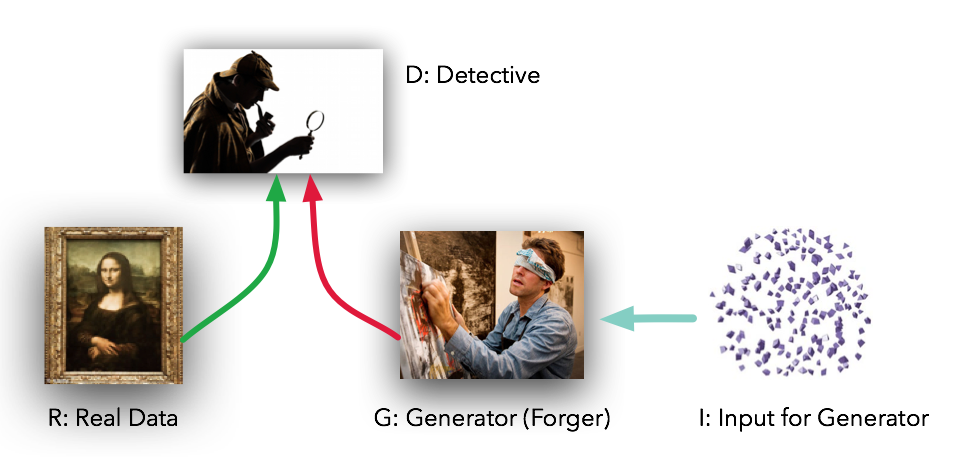
Imagine an art forger that is trying to create fake pieces of art, and an art critic that needs to distinguish between proper paintings and fake ones.

In this scenario, the critic acts like our discriminator, and the forger is the generator, taking feedback from the critic to improve his skills and make his forged art look more convincing:

Training

Training a GAN can be a painful thing. Training instability has always been an issue, and a lot of research has been focusing on making training more stable.

The basic objective function of a vanilla GAN model is the following:

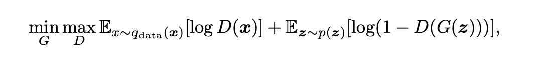
Here, D refers to the discriminator network, while G obviously refers to the generator.

As the formula shows, the generator optimizes for maximally confusing the discriminator, by trying to make it output high probabilities for fake data samples.

On the contrary, the discriminator tries to become better at distinguishing samples coming from G from samples coming from the real distribution.

The term adversarial comes exactly from the way GANS are trained, pitting the two networks against each other.

Once we've trained our model, the discriminator is no longer required. All we have to do is feed the generator a random noise vector, and we'll hopefully get a realistic, artificial data sample as a result.

GANs Issues

So, why are GANs so hard to train? As stated earlier, GANs are very hard to train in their vanilla form. We'll briefly look at why this is the case.

Hard-to-Reach Nash Equilibrium

Since these two networks shoot information at each other, it could be portrayed as a game where one guesses if the input is real or not.

The GAN framework is a non-convex, two-player, non-cooperative game with continuous, high-dimensional parameters, in which each player wants to minimize its cost function. The optimum of this process takes the name of Nash Equilibrium - where each player will not perform any better by changing a strategy, given the fact that the other player doesn't change their strategy.

However, GANs are typically trained using gradient-descent techniques that are designed to find the low value of a cost function and not find the Nash Equilibrium of a game.

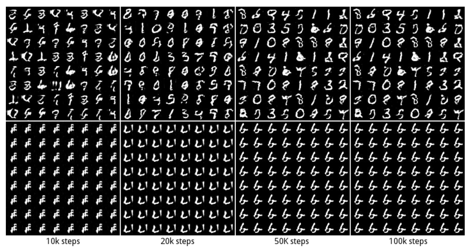
Mode Collapse

Most data distributions are multi-modal. Take the MNIST dataset: there are 10 "modes" of data, referring to the different digits between 0 and 9.

A good generative model would be able to produce samples with sufficient variability, thus being able to generate samples from all the different classes.

However, this does not always happen.

Let's say the the generator becomes really good at producing the digit "3". If the produced samples are convincing enough, the discriminator will likely assign them high probabilities.

As a result, the generator will be pushed towards producing samples that come from that specific mode, ignoring the other classes most of the time. It will essentially spam the same number and with each number that passes the discriminator, this behavior will only further be enforced.

Diminishing Gradient

Very similar to the previous example, the discriminator may get too successful in distinguishing data samples. When that is true, the generator gradient vanishes, it starts learning less and less, failing to converge.

This imbalance, the same as the previous one, can be caused if we train the networks separately. Neural network evolution can be quite unpredictable, which can lead to one being ahead of the other by a mile. If we train them together, we mostly ensure that these things don't happen.

State-of-the-Art

It would be impossible to give a comprehensive view of all the improvements and developments that made GANs more powerful and stable in the past years.

What I'll do instead is compile a list of the most successful architectures and techniques, providing links to relevant resources to go more in depth.

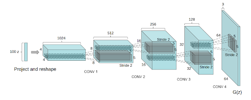
DCGANs

Deep Convolutional GANs (DCGANs) introduced convolutions to the generator and discriminator networks.

However, this was not simply a matter of adding convolutional layers to the model, since training became even more unstable.

Several tricks had to be applied to make DCGANs useful:

• Batch normalization was applied to both the generator and the discriminator network
• Dropout is used as a regularization technique
• The generator needed a way to upsample the random input vector to an output image. Transposing convolutional layers is employed here
• LeakyRelu and TanH activations are used throughout both networks

WGANs

Wasserstein GANs (WGANs) are aimed at improving training stability. There is a heavy amount of math behind this type of model. A more approachable explanation can be found here.

The basic idea here was to propose a new cost function that has a smoother gradient everywhere.

The new cost function uses a metric called Wasserstein distance, that has a smoother gradient everywhere.

As a result, the discriminator, which is now called critic, outputs confidence values which are no longer to be interpreted as a probability. High values mean that the model is confident that the input is a real one.

Two significant improvements for WGAN are:

• It has no sign of mode collapse in experiments
• The generator can still learn when the critic perform well

SAGANs

Self-Attention GANs (SAGANs) introduce an attention mechanism to the GAN framework.

Attention mechanisms allow to use global information locally. What this means is that we can capture meaning from different parts of an image, and use that information to produce better samples.

This comes from the observation that convolutions are quite bad at capturing long-term dependencies in input samples, as the convolution is a local operation whose receptive field depends on the spatial size of the kernel.

This means that, for example, it is not possible for an output on the top-left position of an image to have any relation to the output at bottom-right.

One way to solve this problem would be to use kernels with larger sizes, in order to capture more information. However, this would cause the model to be computationally inefficient, and very slow to train.

Self-attention solves this issue, providing an efficient way to capture global information, and use it locally when it might prove useful.

BigGANs

BigGANs are, at the time of writing, considered more or less state-of-the-art, as far as quality of generated samples is concerned.

What researchers did here was to put together everything that had been working up to that point, and then scaling it up massively.
Their baseline model was in fact a SAGAN, to which they added some tricks to improve stability.

They proved that GANs dramatically benefit from scaling, even when no further functional improvements are introduced to the model, as cited in the original paper:

We have demonstrated that Generative Adversarial Networks trained to model natural images of multiple categories highly benefit from scaling up, both in terms of fidelity and variety of the generated samples. As a result, our models set a new level of performance among ImageNet GAN models, improving on the state of the art by a large margin

A Simple GAN in Python

Code Implementation

With all that said, let's go ahead and implement a simple GAN that generates digits from 0-9, a pretty classic example:

import tensorflow as tf
from tensorflow.examples.tutorials.mnist import input_data
import numpy as np
import matplotlib.pyplot as plt
import matplotlib.gridspec as gridspec
import os

# Sample z from uniform distribution
def sample_Z(m, n):
    return np.random.uniform(-1., 1., size=[m, n])

def plot(samples):
    fig = plt.figure(figsize=(4, 4))
    gs = gridspec.GridSpec(4, 4)
    gs.update(wspace=0.05, hspace=0.05)

    for i, sample in enumerate(samples):
        ax = plt.subplot(gs[i])
        plt.axis('off')
        ax.set_xticklabels([])
        ax.set_yticklabels([])
        ax.set_aspect('equal')
        plt.imshow(sample.reshape(28, 28), cmap='Greys_r')

    return fig

We can now define the placeholder for our input samples and noise vectors:

# Input image, for discriminator model.
X = tf.placeholder(tf.float32, shape=[None, 784])

# Input noise for generator.
Z = tf.placeholder(tf.float32, shape=[None, 100])

Now, we define our generator and discriminator networks. They are simple perceptrons with only one hidden layer.

We use relu activations in the hidden layer neurons, and sigmoids for the output layers.

def generator(z):
    with tf.variable_scope("generator", reuse=tf.AUTO_REUSE):
        x = tf.layers.dense(z, 128, activation=tf.nn.relu)
        x = tf.layers.dense(z, 784)
        x = tf.nn.sigmoid(x)
    return x

def discriminator(x):
    with tf.variable_scope("discriminator", reuse=tf.AUTO_REUSE):
        x = tf.layers.dense(x, 128, activation=tf.nn.relu)
        x = tf.layers.dense(x, 1)
        x = tf.nn.sigmoid(x)
    return x

We can now define our models, loss functions and optimizers:

# Generator model
G_sample = generator(Z)

# Discriminator models
D_real = discriminator(X)
D_fake = discriminator(G_sample)


# Loss function
D_loss = -tf.reduce_mean(tf.log(D_real) + tf.log(1. - D_fake))
G_loss = -tf.reduce_mean(tf.log(D_fake))

# Select parameters
disc_vars = [var for var in tf.trainable_variables() if var.name.startswith("disc")]
gen_vars = [var for var in tf.trainable_variables() if var.name.startswith("gen")]

# Optimizers
D_solver = tf.train.AdamOptimizer().minimize(D_loss, var_list=disc_vars)
G_solver = tf.train.AdamOptimizer().minimize(G_loss, var_list=gen_vars)

Finally, we can write our training routine. At each iteration, we perform one step of optimization for the discriminator and one for the generator.

Every 100 iterations we save some generated samples so we can have a look at our progress.

# Batch size
mb_size = 128

# Dimension of input noise
Z_dim = 100

mnist = input_data.read_data_sets('../../MNIST_data', one_hot=True)

sess = tf.Session()
sess.run(tf.global_variables_initializer())

if not os.path.exists('out2/'):
    os.makedirs('out2/')

i = 0

for it in range(1000000):

    # Save generated images every 1000 iterations.
    if it % 1000 == 0:
        samples = sess.run(G_sample, feed_dict={Z: sample_Z(16, Z_dim)})

        fig = plot(samples)
        plt.savefig('out2/{}.png'.format(str(i).zfill(3)), bbox_inches='tight')
        i += 1
        plt.close(fig)


    # Get the next batch of images. Each batch has mb_size samples.
    X_mb, _ = mnist.train.next_batch(mb_size)


    # Run disciminator solver
    _, D_loss_curr = sess.run([D_solver, D_loss], feed_dict={X: X_mb, Z: sample_Z(mb_size, Z_dim)})

    # Run generator solver
    _, G_loss_curr = sess.run([G_solver, G_loss], feed_dict={Z: sample_Z(mb_size, Z_dim)})

    # Print loss
    if it % 1000 == 0:
        print('Iter: {}'.format(it))
        print('D loss: {:.4}'. format(D_loss_curr))

Results and Possible Improvements

During the first iterations, all we see is random noise:

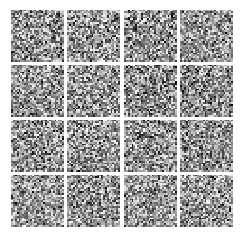
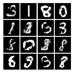
Here, the networks didn't learn anything yet. Though, after only a couple of minutes, we can already see how our digits are taking shape!

Resources

If you'd like to play around with the code, it's up on GitHub!

• Explanation of SAGANs
• Improved techniques for training GANs
• Must-Read Papers on GANs