Introduction to Image Processing in Python with OpenCV

Introduction

In this tutorial, we are going to learn how we can perform image processing using the Python language. We are not going to restrict ourselves to a single library or framework; however, there is one that we will be using the most frequently, the Open CV library. We will start off by talking a little about image processing and then we will move on to see different applications/scenarios where image processing can come in handy. So, let's begin!

What is Image Processing?

It is important to know what exactly image processing is and what is its role in the bigger picture before diving into its how's. Image Processing is most commonly termed as 'Digital Image Processing' and the domain in which it is frequently used is 'Computer Vision'. Don't be confused - we are going to talk about both of these terms and how they connect. Both Image Processing algorithms and Computer Vision (CV) algorithms take an image as input; however, in image processing, the output is also an image, whereas in computer vision the output can be some features/information about the image.

Why do we need it?

The data that we collect or generate is mostly raw data, i.e. it is not fit to be used in applications directly due to a number of possible reasons. Therefore, we need to analyze it first, perform the necessary pre-processing, and then use it.

For instance, let's assume that we were trying to build a cat classifier. Our program would take an image as input and then tell us whether the image contains a cat or not. The first step for building this classifier would be to collect hundreds of cat pictures. One common issue is that all the pictures we have scraped would not be of the same size/dimensions, so before feeding them to the model for training, we would need to resize/pre-process them all to a standard size.

This is just one of many reasons why image processing is essential to any computer vision application.

Prerequisites

Before going any further, let's discuss what you need to know in order to follow this tutorial with ease. Firstly, you should have some basic programming knowledge in any language. Secondly, you should know what machine learning is and the basics of how it works, as we will be using some machine learning algorithms for image processing in this article. As a bonus, it would help if you have had any exposure to, or basic knowledge of, Open CV before going on with this tutorial. But this is not required.

One thing you should definitely know in order to follow this tutorial is how exactly an image is represented in memory. Each image is represented by a set of pixels i.e. a matrix of pixel values. For a grayscale image, the pixel values range from 0 to 255 and they represent the intensity of that pixel. For instance, if you have an image of 20 x 20 dimensions, it would be represented by a matrix of 20x20 (a total of 400-pixel values).

If you are dealing with a colored image, you should know that it would have three channels - Red, Green, and Blue (RGB). Therefore, there would be three such matrices for a single image.

Installation

Note: Since we are going to use OpenCV via Python, it is an implicit requirement that you already have Python (version 3) already installed on your workstation.

Windows

$ pip install opencv-python

MacOS

$ brew install opencv3 --with-contrib --with-python3

Linux

$ sudo apt-get install libopencv-dev python-opencv

To check if your installation was successful or not, run the following command in either a Python shell or your command prompt:

import cv2

Some Basics You Should Know

Before we move on to using Image Processing in an application, it is important to get an idea of what kind of operations fall into this category, and how to do those operations. These operations, along with others, would be used later on in our applications. So, let's get to it.

For this article we'll be using the following image:

Note: The image has been scaled for the sake of displaying it in this article, but the original size we are using is about 1180x786.

You probably noticed that the image is currently colored, which means it is represented by three color channels i.e. Red, Green, and Blue. We will be converting the image to grayscale, as well as splitting the image into its individual channels using the code below.

Finding Image Details

After loading the image with the imread() function, we can then retrieve some simple properties about it, like the number of pixels and dimensions:

import cv2

img = cv2.imread('rose.jpg')

print("Image Properties")
print("- Number of Pixels: " + str(img.size))
print("- Shape/Dimensions: " + str(img.shape))

Output:

Image Properties
- Number of Pixels: 2782440
- Shape/Dimensions: (1180, 786, 3)

Splitting an Image into Individual Channels

Now we'll split the image in to its red, green, and blue components using OpenCV and display them:

from google.colab.patches import cv2_imshow

blue, green, red = cv2.split(img) # Split the image into its channels
img_gs = cv2.imread('rose.jpg', cv2.IMREAD_GRAYSCALE) # Convert image to grayscale

cv2_imshow(red) # Display the red channel in the image
cv2_imshow(blue) # Display the red channel in the image
cv2_imshow(green) # Display the red channel in the image
cv2_imshow(img_gs) # Display the grayscale version of image

For brevity, we'll just show the grayscale image.

Grayscale Image:

Image Thresholding

The concept of thresholding is quite simple. As discussed above in the image representation, pixel values can be any value between 0 to 255. Let's say we wish to convert an image into a binary image i.e. assign a pixel either a value of 0 or 1. To do this, we can perform thresholding. For instance, if the Threshold (T) value is 125, then all pixels with values greater than 125 would be assigned a value of 1, and all pixels with values lesser than or equal to that would be assigned a value of 0. Let's do that through code to get a better understanding.

Image used for Thresholding:

import cv2

# Read image
img = cv2.imread('image.png', 0)

# Perform binary thresholding on the image with T = 125
r, threshold = cv2.threshold(img, 125, 255, cv2.THRESH_BINARY)
cv2_imshow(threshold)

Output:

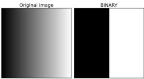
As you can see, in the resultant image, two regions have been established, i.e. the black region (pixel value 0) and white region (pixel value 1). Turns out, the threshold we set was right in the middle of the image, which is why the black and white values are divided there.

Applications

#1: Removing Noise from an Image

Now that you have got a basic idea of what image processing is and what it is used for, let's go ahead and learn about some of its specific applications.

In most cases, the raw data that we gather has noise in it i.e. unwanted features that makes the image hard to perceive. Although these images can be used directly for feature extraction, the accuracy of the algorithm would suffer greatly. This is why image processing is applied to the image before passing it to the algorithm to get better accuracy.

There are many different types of noise, like Gaussian noise, salt and pepper noise, etc. We can remove that noise from an image by applying a filter which removes that noise, or at the very least, minimizes its effect. There are a lot of options when it comes to filters as well, each of them has different strengths, and hence is the best for a specific kind of noise.

To understand this properly, we are going to add 'salt and pepper' noise to the grayscale version of the rose image that we considered above, and then try to remove that noise from our noisy image using different filters and see which one is best-fit for that type.

import numpy as np

# Adding salt & pepper noise to an image
def salt_pepper(prob):
      # Extract image dimensions
      row, col = img_gs.shape

      # Declare salt & pepper noise ratio
      s_vs_p = 0.5
      output = np.copy(img_gs)

      # Apply salt noise on each pixel individually
      num_salt = np.ceil(prob * img_gs.size * s_vs_p)
      coords = [np.random.randint(0, i - 1, int(num_salt))
            for i in img_gs.shape]
      output[coords] = 1

      # Apply pepper noise on each pixel individually
      num_pepper = np.ceil(prob * img_gs.size * (1. - s_vs_p))
      coords = [np.random.randint(0, i - 1, int(num_pepper))
            for i in img_gs.shape]
      output[coords] = 0
      cv2_imshow(output)

      return output

# Call salt & pepper function with probability = 0.5
# on the grayscale image of rose
sp_05 = salt_pepper(0.5)

# Store the resultant image as 'sp_05.jpg'
cv2.imwrite('sp_05.jpg', sp_05)

Alright, we have added noise to our rose image, and this is what it looks like now:

Noisy Image:

Lets now apply different filters on it and note down our observations i.e. how well each filter reduces the noise.

Arithmetic Filter with Sharpening Kernel

# Create our sharpening kernel, the sum of all values must equal to one for uniformity
kernel_sharpening = np.array([[-1,-1,-1],
                              [-1, 9,-1],
                              [-1,-1,-1]])

# Applying the sharpening kernel to the grayscale image & displaying it.
print("\n\n--- Effects on S&P Noise Image with Probability 0.5 ---\n\n")

# Applying filter on image with salt & pepper noise
sharpened_img = cv2.filter2D(sp_05, -1, kernel_sharpening)
cv2_imshow(sharpened_img)

The resulting image, from applying arithmetic filter on the image with salt and pepper noise, is shown below. Upon comparison with the original grayscale image, we can see that it brightens the image too much and is unable to highlight the bright spots on the rose as well. Hence, it can be concluded that arithmetic filter fails to remove salt and pepper noise.

Arithmetic Filter Output:

Midpoint Filter

from scipy.ndimage import maximum_filter, minimum_filter

def midpoint(img):
    maxf = maximum_filter(img, (3, 3))
    minf = minimum_filter(img, (3, 3))
    midpoint = (maxf + minf) / 2
    cv2_imshow(midpoint)

print("\n\n---Effects on S&P Noise Image with Probability 0.5---\n\n")
midpoint(sp_05)

The resulting image, from applying th Midpoint Filter on the image with salt and pepper noise, is shown below. Upon comparison with the original grayscale image, we can see that, like the kernel method above, brightens the image too much; however, it is able to highlight the bright spots on the rose. Therefore, we can say that it is a better choice than the arithmetic filter, but still it does not recover the original image completely.

Midpoint Filter Output:

Contraharmonic Mean Filter

Note: The implementations of these filters can be found online easily and how exactly they work is out of scope for this tutorial. We will be looking at the applications from an abstract/higher level.

def contraharmonic_mean(img, size, Q):
    num = np.power(img, Q + 1)
    denom = np.power(img, Q)
    kernel = np.full(size, 1.0)
    result = cv2.filter2D(num, -1, kernel) / cv2.filter2D(denom, -1, kernel)
    return result

print("\n\n--- Effects on S&P Noise Image with Probability 0.5 ---\n\n")
cv2_imshow(contraharmonic_mean(sp_05, (3,3), 0.5))

The resulting image, from applying Contraharmonic Mean Filter on the image with salt and pepper noise, is shown below. Upon comparison with the original grayscale image, we can see that it has reproduced pretty much the exact same image as the original one. Its intensity/brightness level is the same and it highlights the bright spots on the rose as well. Hence, we can conclude that contraharmonic mean filter is very effective in dealing with salt and pepper noise.

Contraharmonic Mean Filter Output:

Now that we have found the best filter to recover the original image from a noisy one, we can move on to our next application.

#2: Edge Detection using Canny Edge Detector

The rose image that we have been using so far has a constant background i.e. black, therefore, we will be using a different image for this application to better show the algorithm's capabilities. The reason is that if the background is constant, it makes the edge detection task rather simple, and we don't want that.

We talked about a cat classifier earlier in this tutorial, let's take that example forward and see how image processing plays an integral role in that.

In a classification algorithm, the image is first scanned for 'objects' i.e. when you input an image, the algorithm would find all the objects in that image and then compare them against the features of the object that you are trying to find. In case of a cat classifier, it would compare all objects found in an image against the features of a cat image, and if a match is found, it tells us that the input image contains a cat.

Since we are using the cat classifier as an example, it is only fair that we use a cat image going forward. Below is the image we will be using:

Image used for Edge Detection:

import cv2
import numpy as np
from matplotlib import pyplot as plt

# Declaring the output graph's size
plt.figure(figsize=(16, 16))

# Convert image to grayscale
img_gs = cv2.imread('cat.jpg', cv2.IMREAD_GRAYSCALE)
cv2.imwrite('gs.jpg', img_gs)

# Apply canny edge detector algorithm on the image to find edges
edges = cv2.Canny(img_gs, 100,200)

# Plot the original image against the edges
plt.subplot(121), plt.imshow(img_gs)
plt.title('Original Gray Scale Image')
plt.subplot(122), plt.imshow(edges)
plt.title('Edge Image')

# Display the two images
plt.show()

Edge Detection Output:

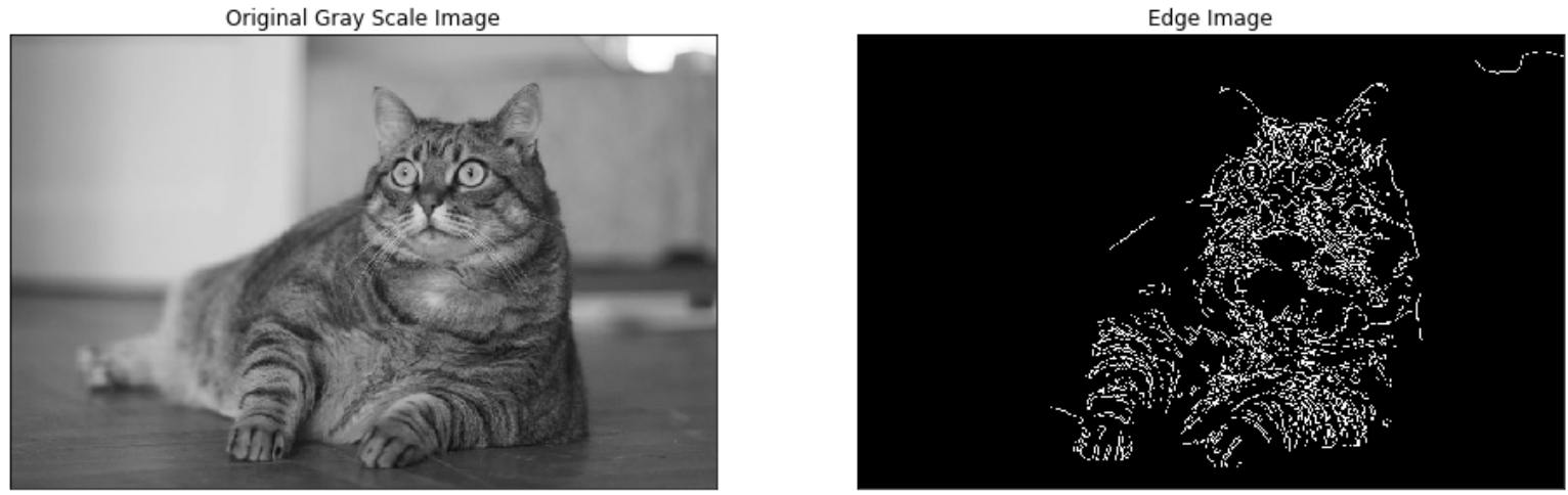
As you can see, the part of the image which contains an object, which in this case is a cat, has been dotted/separated through edge detection. Now you must be wondering, what is the Canny Edge Detector and how did it make this happen; so let's discuss that now.

To understand the above, there are three key steps that need to be discussed. First, it performs noise reduction on the image in a similar manner that we discussed previously. Second, it uses the first derivative at each pixel to find edges. The logic behind this is that the point where an edge exists, there is an abrupt intensity change, which causes a spike in the first derivative's value, hence making that pixel an 'edge pixel'.

At the end, it performs hysteresis thresholding; we said above that there's a spike in the value of first derivative at an edge, but we did not state 'how high' the spike needs to be for it to be classified as an edge - this is called a threshold! Earlier in this tutorial we discussed what simple thresholding is. Hysteresis thresholding is an improvement on that, it makes use of two threshold values instead of one. The reason behind that is, if the threshold value is too high, we might miss some actual edges (true negatives) and if the value is too low, we would get a lot of points classified as edges that actually are not edges (false positives). One threshold value is set high, and one is set low. All points which are above the 'high threshold value' are identified as edges, then all points which are above the low threshold value but below the high threshold value are evaluated; the points which are close to, or are neighbors of, points which have been identified as edges, are also identified as edges and the rest are discarded.

These are the underlying concepts/methods that Canny Edge Detector algorithm uses to identify edges in an image.

Conclusion

In this article, we learned how to install OpenCV, the most popular library for image processing in Python, on different platforms like Windows, MacOS, and Linux, as well as how to verify that the installation was successful.

We went on to discuss what Image Processing is and its uses in the computer vision domain of Machine Learning. We talked about some common types of noise and how we can remove it from our images using different filters, before using the images in our applications.

Furthermore, we learned how image processing plays an integral part in high-end applications like Object Detection or classification. Do note that this article was just the tip of the iceberg, and Digital Image Processing has a lot more in the store that cannot possibly be covered in a single tutorial. Reading this should enable you to dive deeper and learn about other advanced concepts related to image processing. Good Luck!