Multiple Linear Regression with Python

Introduction

Linear regression is one of the most commonly used algorithms in machine learning. You'll want to get familiar with linear regression because you'll need to use it if you're trying to measure the relationship between two or more continuous values.

A deep dive into the theory and implementation of linear regression will help you understand this valuable machine learning algorithm.

Defining Terms

Before we delve into linear regression, let's take a moment to make sure we are clear on what regression is.

In machine learning, there are two different types of supervised learning methods: classification and regression.

In general, regression is a statistical method that estimates relationships between variables. Classification also attempts to find relationships between variables, with the main difference between classification and regression being the output of the model.

In a regression task, the output variable is numerical or continuous in nature, while for classification tasks the output variable is categorical or discrete in nature. If a variable is categorical it means that there is a finite/discrete number of groups or categories the variable can fit into.

Consider a classifier that tries to predict what type of mammal an animal is, based on different features. Although there are many mammals, there are not infinite mammals, there are only so many possible categories the output can be classified into.

In contrast, continuous variables will have an infinite number of values between any two variables. The difference between two given numbers can be represented as an infinite number of ways, writing out ever longer decimals. This means that even things like date and time measurements can be considered continuous variables if the measurements are not put into discrete categories.

While regression tasks are concerned with estimating the relationship between some input variable with a continuous output variable, there are different types of regression algorithms:

• Linear regression
• Polynomial regression
• Stepwise regression
• Ridge regression
• Lasso regression
• ElasticNet regression

These different types of regression are suitable for different tasks. Ridge regression is best used when there are high degrees of collinearity or nearly linear relationships in the set of features. Meanwhile, Polynomial regression is best used when there is a non-linear relationship between features, as it is capable of drawing curved prediction lines.

Linear regression is one of the most commonly used regression types, suited for drawing a straight line across a graph that shows a linear relationship between variables.

Theory Behind Multiple Linear Regression

A linear regression simply shows the relationship between the dependent variable and the independent variable.

If linear regression is just the plotting of a relationship between an independent variable (X) and a dependent variable (Y), you may be able to guess that multivariate/multiple linear regression is just a linear regression carried out on more than one independent variable.

Let's take a look at the equation for linear regression, as understanding how it works will assist you in knowing when to apply it.

Credit: commons.wikimedia.org

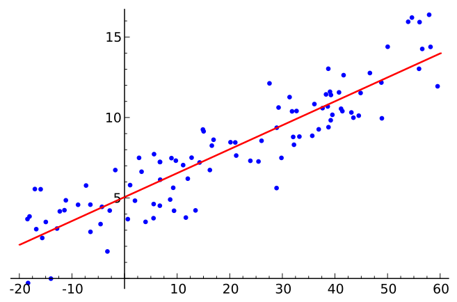
The equation for linear regression is: Y = a+b*X. In a linear regression task we will have the parameters (a and b) be estimated by our model. We will then take the constant, or intercept a, and add the slope of the line b times the independent variable X (our input feature), to figure out the value of the dependent variable (Y).

The picture above is an example of what a linear relationship between the X and Y variables look like.

The equation used to calculate the values of a and b for the best fit line is the Least Square Method, which functions by minimizing squared distance from each data point to the line being drawn. You don't need to know how the equation works exactly to implement Linear Regression, but if you are curious you can read more about it in the link above.

If Y = a+b*X is the equation for singular linear regression, then it follows that for multiple linear regression, the number of independent variables and slopes are plugged into the equation.

For instance, here is the equation for multiple linear regression with two independent variables:

$$Y=a+b1\ast X1+b2\ast x2$$

This holds true for any given number of variables.

Multivariate linear regression can be thought as multiple regular linear regression models, since you are just comparing the correlations between between features for the given number of features.

For the equations mentioned above, it is assumed that there is a linear relationship between the dependent variable and the independent variable or variables. This also assumes that the variables/features are all continuous values rather than discrete values.

Implementing MLR

Converting Categorical Variables

Credit: commons.wikimedia.org

When implementing linear regression in a machine learning system, the variables must be continuous in nature, not categorical. However, you will frequently have data that contains categorical variables and not continuous variables.

For instance, a dataset could contain occurrences of some event in specific countries. The countries are categorical variables. In order to properly use linear regression, these categorical variables must be converted into continuous variables.

There are several different ways that this can be achieved, depending on the type of variable in question. Variables can be either dichotomous, nominal, or ordinal.

Dichotomous Variables

Dichotomous variables are those which exist in only one of two categories. A dichotomous variable is either "yes" or "no", white or black. Dichotomous variables are easy to convert into continuous variables, they simply must be labeled 0 or 1.

Nominal/Ordinal Variables

Nominal and ordinal variables are types of categorical variables, and there can be any number of categories the values can belong to. In terms of ordinal variables, it is assumed that there is some order to the variables, or that the variables should have different weights. Therefore, the categorical variables can be converted into continuous values by assigning them numbers starting at zero and running until the length of the categories.

Converting nominal variables into continuous variables is the most challenging task out of all three types of conversion. This is because nominal variables should not have a different weight or order attached to them, it is presumed that all categorical variables have equivalent "values". This means that you cannot simply order them from zero to the number of categories as this would imply that the earlier categories have less "value" than later categories.

For this reason, the default tactic for transforming nominal variables into continuous variables is something called one-hot encoding, sometimes referred to as "creating dummy variables". Essentially, you create more features or variables that stand in for the actual categories in your data. The process of one-hot encoding means creating an array the size of your number of categories and filling them in with a "one" in the position corresponding to the relevant category and zeros everywhere else.

For an example, here's a table with categorical data:

Color
Red
Green
Blue

After we put this table through the one-hot-encoding process, it ends up looking like this:

Red	Green	Blue
1	0	0
0	1	0
0	0	1

When you are creating continuous labels for your categorical variables, be sure that the values genuinely correspond to the significance of the category in question. If you have ordinal variables and the range of values you're given, don't keep the rank in mind, the relationships between the categories will be lost and your classifier will be adversely affected.

Machine Learning Pipeline

Before we look at an example of implementing multiple linear regression on an actual data set, let's take a moment to understand the machine learning workflow or pipeline.

Every implementation of machine learning algorithms has the same basic components. You need to:

• Prepare the data
• Create the model
• Train the model
• Evaluate the model

Preparing the data is frequently one of the most challenging parts of machine learning, as it involves not only collecting the data but then transforming that data into a format that can be utilized by your chosen algorithm. This involves many tasks like dealing with missing values or corrupted/malformed data. For this reason, we will be using a pre-made data set that requires little preprocessing.

Creating the machine learning model is fairly straightforward when using a library like Scikit-Learn. There are typically only a few lines of code necessary to instantiate a given machine learning algorithm. However, there are different arguments and parameters these algorithms take that will affect your model's accuracy. The art of choosing the correct parameter values for the model will come to you over time, but you can always refer to the algorithm's documentation in your chosen library to see which parameters you can experiment with.

Training the model is also rather straight-forward when using a library like Scikit-Learn, as once more there are usually only a few lines of code needed to train the algorithm on your chosen data set.

However, you must be sure you have divided your data into training and testing sets. You cannot evaluate the performance of your classifier on the same data set you have trained it on, as your model has already learned the parameters of this set of data. Evaluating the data on the training set won't give you any insight regarding your model's performance on another data set.

Sample MLR Implementation

Without further delay, let's examine how to carry out multiple linear regression using the Scikit-Learn module for Python.

Credit: commons.wikimedia.org

First, we need to load in our dataset. We're using the Scikit-Learn library, and it comes prepackaged with some sample datasets. The dataset we'll be using is the Boston Housing Dataset. The dataset has many different features about homes in the Boston area, like house size, crime rate, building age, etc. The goal is to predict the price of the house based on these features.

Here are all the imports we need:

import numpy as np
import pandas as pd
from sklearn.model_selection import train_test_split
from sklearn.datasets import load_boston
from sklearn.metrics import mean_squared_error, r2_Score

We now need to create an instance of the dataset, by calling the load_boston() function:

bh_data = load_boston()

Let's print out the value of the data variable to see what kinds of data it contains:

print(bh_data.keys())

Here's what we get back:

dict_keys(['data', 'target', 'feature_names', 'DESCR'])

The data is all the actual information regarding the houses, while the target is the price of the house, the feature names are the names of the categories the data falls into, and DESCR is a command to describe the features of the dataset.

We're trying to get the data and the feature names into a dataframe our model can use, so let's create a dataframe object from the data using Pandas.

We also pass in the feature names as column headers:

boston = pd.Dataframe(bh_data.data, columns=bh_data.feature_names)

If we want to get an idea of the kinds of features in the dataset, we can print out some of the rows, along with a description of what the features are:

print(data.DESCR)

Here's a few of the descriptions that are returned:

CRIM: Per capita crime rate by town
ZN: Proportion of residential land zoned for lots over 25,000 sq. ft
INDUS: Proportion of non-retail business acres per town
...
LSTAT: Percentage of lower status of the population
MEDV: Median value of owner-occupied homes in $1000s

We want to predict the median value of a home, but our current dataset doesn't have that information to train/test on, so let's create a new column in the dataframe and load in the target values from the dataset.

This is done just by specifying the data frame and the name of the column we want to create in the variable, then selecting the target values:

boston['MEDV'] = bh_data.target

Normally, you would do some data analysis to figure out what the most important features are and use those variables for the regression. That could be an article all by itself, however, so in this case, I'll just tell you that the features with the strongest correlations are the proportion of "lower status" in the population ('LSTAT') and the number of rooms in the house ('RM').

So let's use 'RM' and 'LSTAT' as our variables for linear regression. These values are already continuous in our dataset, so we don't need to encode them at all.

However, let's concatenate the two variable columns into a single column with the NumPy library's np.c_ command. We'll also create a new variable to store the target values by specifying the boston dataframe and the column we want:

X = pd.DataFrame(np.c_[boston['LSTAT'], boston['RM']], columns=['LSTAT','RM']
Y = boston['MEDV']

Now let's split the dataframe into training and testing sets:

X_train, X_test, y_train, y_test = train_test_split(X, y, test_size = 0.2, random_state=9)

We now need to create an instance of the model, which we do simply calling the LinearRegression function from Scikit-Learn:

lin_reg_mod = LinearRegression()

We now fit the model on the training data:

lin_reg_mod.fit(X_train, y_train)

Now that the model has been fit we can make predictions by calling the predict command. We are making predictions on the testing set:

pred = lin_reg_mod.predict(X_test)

We'll now check the predictions against the actual values by using the RMSE and R-2 metrics, two metrics commonly used to evaluate regression tasks:

test_set_rmse = (np.sqrt(mean_squared_error(y_test, pred)))

test_set_r2 = r2_score(y_test, pred)

Excellent. There are our variables storing the evaluation of the model, and we have a complete implementation of multiple linear regression on a sample dataset.

Let's print out the accuracy metrics and see what results we get:

print(test_set_rmse)
print(test_set_r2)

Here are our results:

# Note that for rmse, the lower that value is, the better the fit
6.035041736063677
# The closer towards 1, the better the fit
0.6400551238836978

You could try using more features to improve the accuracy of the model.

Conclusion

Multivariate/multiple linear regression is an extremely useful algorithm for tracking the relationships of continuous variables. It is also one of the most commonly used algorithms in machine learning, so it pays to familiarize yourself with it.