Introduction
Internet marketing has taken over traditional marketing strategies in the recent past. Companies prefer to advertise their products on websites and social media platforms. However, targeting the right audience is still a challenge in online marketing. Spending millions to display the advertisement to the audience that is not likely to buy your products can be costly. One effective strategy to consider is affiliate marketing, which allows companies to reach specific demographics through trusted affiliates.
In this article, we will work with the advertising data of a marketing agency to develop a machine learning algorithm that predicts if a particular user will click on an advertisement. The data consists of 10 variables: Daily Time Spent on Site, Age, Area Income, Daily Internet Usage, Ad Topic Line, City, Male, Country, Timestamp and Clicked on Ad.
The main variable we are interested in is 'Clicked on Ad'. This variable can have two possible outcomes: 0 and 1 where 0 refers to the case where a user didn't click the advertisement, while 1 refers to the scenario where a user clicks the advertisement.
We will see if we can use the other 9 variables to accurately predict the value 'Clicked on Ad' variable. We will also perform some exploratory data analysis to see how Daily Time Spent on Site in combination with Ad Topic Line affects the user's decision to click on the ad.
Importing Libraries
To develop our prediction model, we need to import the necessary Python libraries:
import pandas as pd
import numpy as np
import matplotlib.pyplot as plt
import seaborn as sns

%matplotlib inline
Importing the Dataset
The dataset for this article can be downloaded from this Kaggle link. Unzip the downloaded zip file and place the advertising.csv file in your local drive. This is the file that we are going to use to train our machine learning model.
Now we need to load the data:
data = pd.read_csv('E:/Datasets/advertising.csv')
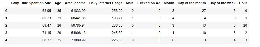
Let's see the first ten lines of our DataFrame:
data.head(10)
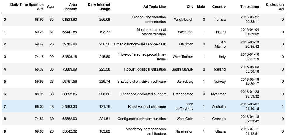
Based on the first lines in the table, we can get a basic insight into the data we are working with. We want to check how much data we have within each variable.
data.info()
Output:
<class 'pandas.core.frame.DataFrame'>
RangeIndex: 1000 entries, 0 to 999
Data columns (total 10 columns):
Daily Time Spent on Site    1000 non-null float64
Age                         1000 non-null int64
Area Income                 1000 non-null float64
Daily Internet Usage        1000 non-null float64
Ad Topic Line               1000 non-null object
City                        1000 non-null object
Male                        1000 non-null int64
Country                     1000 non-null object
Timestamp                   1000 non-null object
Clicked on Ad               1000 non-null int64
dtypes: float64(3), int64(3), object(4)
memory usage: 78.2+ KB
Good news! All variables are complete and there are no missing values within them. Each of them contains 1000 elements and there will be no need for additional preprocessing of raw data.
We will also use the describe function to gain insight into the ranges in which variables change:
data.describe()
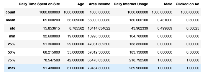
An interesting fact from the table is that the smallest area income is $13,996.50 and the highest is $79,484.80. This means that site visitors are people belonging to different social classes. It can also be concluded that we are analyzing a popular website since users spend between 32 and 91 minutes on the website in one session. These are really big numbers!
Furthermore, the average age of a visitor is 36 years. We see that the youngest user is 19 and the oldest is 61 years old. We can conclude that the site is targeting adult users. Finally, if we are wondering whether the site is visited more by men or women, we can see that the situation is almost equal (52% in favor of women).
To further analyze our data, let's first plot a histogram with Kernel density estimation for the Age variable.
from scipy.stats import norm
sns.distplot(data['Age'], hist=False, color='r', rug=True, fit=norm);
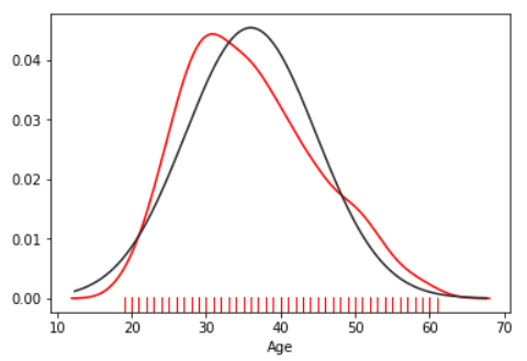
It can be concluded that the variable Age has a normal distribution of data. We will see in some of the following articles why this is good for effective data processing.
Let's plot a two-dimensional density plot to determine the interdependence of two variables. Let's see how the user's age and the time spent on the site are linked.
f, ax = plt.subplots(figsize=(10, 10))
sns.kdeplot(data.Age, data['Daily Time Spent on Site'], color="b", ax=ax)
sns.rugplot(data.Age, color="r", ax=ax)
sns.rugplot(data['Daily Time Spent on Site'], vertical=True, ax=ax)
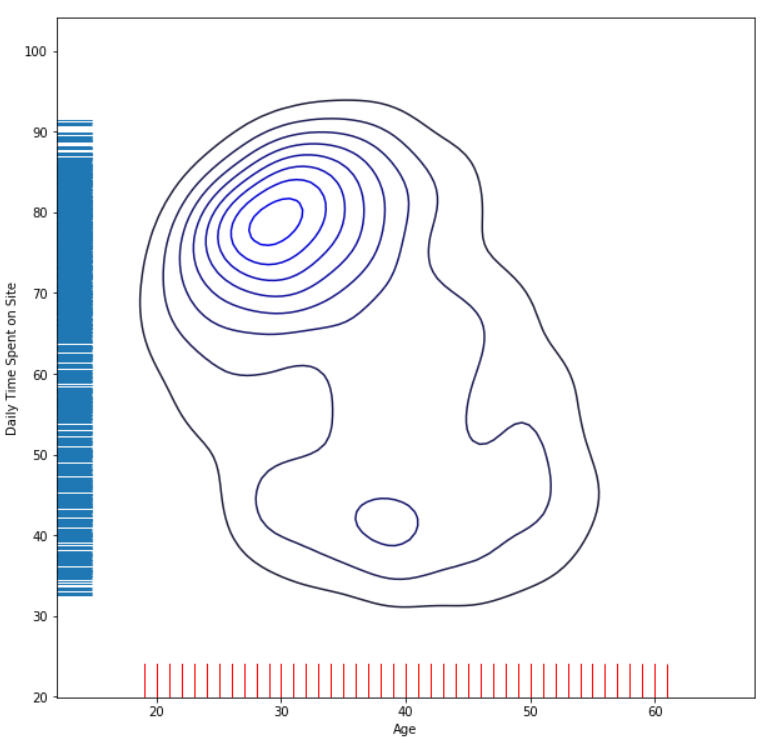
From the picture, we can conclude that younger users spend more time on the site. This implies that users of the age between 20 and 40 years can be the main target group for the marketing campaign. Hypothetically, if we have a product intended for middle-aged people, this is the right site for advertising. Conversely, if we have a product intended for people over the age of 60, it would be a mistake to advertise on this site.
We will present another density graphic and determine the interdependency of Daily Time Spent on Site and Daily Internet Usage.
f, ax = plt.subplots(figsize=(8, 8))
cmap = sns.cubehelix_palette(as_cmap=True, start=0, dark=0, light=3, reverse=True)
sns.kdeplot(data["Daily Time Spent on Site"], data['Daily Internet Usage'],
    cmap=cmap, n_levels=100, shade=True);
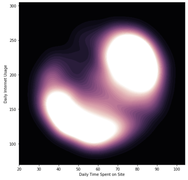
Check out our hands-on, practical guide to learning Git, with best-practices, industry-accepted standards, and included cheat sheet. Stop Googling Git commands and actually learn it!
From the figure above, it is clear that users who spend more time on the internet also spend more time on the site.
Now we will show how to visualize trends in the data using the scatter_matrix function. We will include only numerical variables for performing analysis.
from pandas.plotting import scatter_matrix
scatter_matrix(data[['Daily Time Spent on Site', 'Age','Area Income', 'Daily Internet Usage']],
    alpha=0.3, figsize=(10,10))
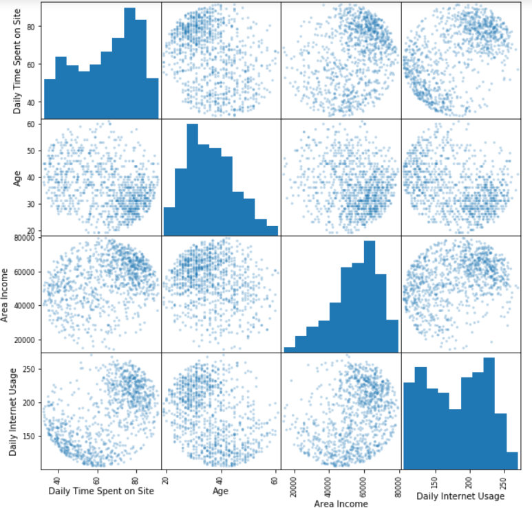
The big picture gives a good insight into the properties of the users who click on the advertisements. On this basis, a large number of further analyzes can be made. We leave them to you, try to find other interesting facts from the data and share it with us in the comments.
Data Preprocessing
You may have noticed that Ad Topic Line, City, and Country are categorical columns. Let's plot all the unique values for these columns.
object_variables = ['Ad Topic Line', 'City', 'Country']
data[object_variables].describe(include=['O'])
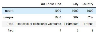
As we can see from the table above, all the values in column Ad Topic Line are unique, while the City column contains 969 unique values out of 1000. There are too many unique elements within these two categorical columns and it is generally difficult to perform a prediction without the existence of a data pattern. Because of that, they will be omitted from further analysis. The third categorical variable, i.e Country, has a unique element (France) that repeats 9 times. Additionally, we can determine countries with the highest number of visitors:
pd.crosstab(index=data['Country'], columns='count').sort_values(['count'], ascending=False).head(20)
The table below shows the 20 most represented countries in our DataFrame.
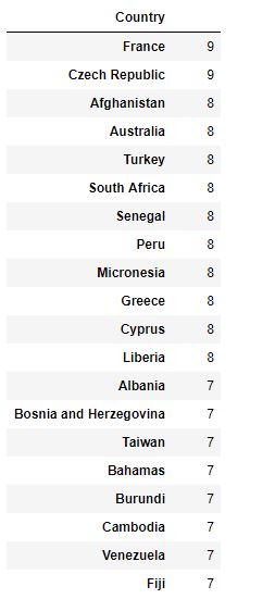
We have already seen, there are 237 different unique countries in our dataset and no single country is too dominant. A large number of unique elements will not allow a machine learning model to establish easily valuable relationships. For that reason, this variable will be excluded too.
data = data.drop(['Ad Topic Line', 'City', 'Country'], axis=1)
Next, we will analyze the 'Timestamp' category. It represents the exact time when a user clicked on the advertisement. We will expand this category to 4 new categories: month, day of the month, day of the week, and hour. In this way, we will get new variables that an ML model will be able to process and find possible dependencies and correlations. Since we have created new variables, we will exclude the original variable "Timestamp" from the table. The "Day of the week" variable contains values from 0 to 6, where each number represents a specific day of the week (from Monday to Sunday).
data['Timestamp'] = pd.to_datetime(data['Timestamp'])

data['Month'] = data['Timestamp'].dt.month
data['Day of the month'] = data['Timestamp'].dt.day
data["Day of the week"] = data['Timestamp'].dt.dayofweek
data['Hour'] = data['Timestamp'].dt.hour
data = data.drop(['Timestamp'], axis=1)

data.head()
Train and Test Data Sets
Once the dataset is processed, we need to divide it into two parts: training and test set. We will import and use the train_test_split function for that. All variables except 'Clicked on Ad' will be the input values X for the ML models. The variable 'Clicked on Ad' will be stored in y, and will represent the prediction variable. We arbitrarily chose to allocate 33% of the total data for the training set.
from sklearn.model_selection import train_test_split

X = data[['Daily Time Spent on Site', 'Age', 'Area Income', 'Daily Internet Usage',
    'Male', 'Month', 'Day of the month' ,'Day of the week']]
y = data['Clicked on Ad']
X_train, X_test, y_train, y_test = train_test_split(X, y, test_size=0.33, random_state=42)
Model Development and Fitting Procedures
In this article, two different ML models will be developed: a Logistic Regression model and a Decision Tree model.
The Logistic Regression model is an algorithm that uses a logistic function to model binary dependent variables. It is a tool for predictive analysis and it is used to explain the relationships between multiple variables. You can find out more about this technique at the following link: Logistic Regression.
The Decision Tree is one of the most commonly used data mining techniques for analysis and modeling. It is used for classification, prediction, estimation, clustering, data description, and visualization. The advantages of Decision Trees, compared to other data mining techniques are simplicity and computation efficiency. Some background on decision trees and how to use them with Scikit-Learn can be found here: Decision Trees in Python with Scikit-Learn
The first model we will import will be a Logistic Regression model. First, it is necessary to load the LogisticRegression function from the sklearn.linear_model library. Also, we will load the accuracy_score to evaluate the classification performances of the model.
from sklearn.linear_model import LogisticRegression
from sklearn.metrics import accuracy_score
from sklearn.metrics import confusion_matrix
The next steps are the initialization of the model, its training, and finally, making predictions.
model_1 = LogisticRegression(solver='lbfgs')
model_1.fit(X_train, y_train)
predictions_LR = model_1.predict(X_test)

print('Logistic regression accuracy:', accuracy_score(predictions_LR, y_test))
print('')
print('Confusion matrix:')
print(confusion_matrix(y_test,predictions_LR))
Output:
Logistic regression accuracy: 0.906060606060606

Confusion matrix:
[[158   4]
 [ 27 141]]
The accuracy of the logistic regression model is 0.906 or 90.6%. As can be observed, the performance of the model is also determined by the confusion matrix. The condition for using this matrix is to be exploited on a data set with known true and false values. You can find additional information on the confusion matrix here: Confusion Matrix.
Our confusion matrix tells us that the total number of accurate predictions is 158 + 141 = 299. On the other hand, the number of incorrect predictions is 27 + 4 = 31. We can be satisfied with the prediction accuracy of our model.
Now we will import DecisionTreeClassifier from the sklearn.tree library. model_2 will be based on the decision tree technique, it will be trained as in the previous case, and desired predictions will be made.
from sklearn.tree import DecisionTreeClassifier

model_2 = DecisionTreeClassifier()
model_2.fit(X_train, y_train)
predictions_DT = model_2.predict(X_test)

print('Decision tree accuracy:', accuracy_score(predictions_DT, y_test))
print('')
print('Confusion matrix:')
print(confusion_matrix(y_test,predictions_DT))
Output:
Decision tree accuracy: 0.9333333333333333

Confusion matrix:
[[151  11]
 [ 11 157]]
It can be concluded that the Decision Tree model showed better performances in comparison to the Logistic Regression model. The confusion matrix shows us that the 308 predictions have been done correctly and that there are only 22 incorrect predictions. Additionally, Decision Tree accuracy is better by about 3% in comparison to the first regression model.
Conclusion
The obtained results showed the use value of both machine learning models. The Decision Tree model showed slightly better performance than the Logistic Regression model, but definitely, both models have shown that they can be very successful in solving classification problems.
The prediction results can certainly be changed by a different approach to data analysis. We encourage you to do your analysis from the beginning, to find new dependencies between variables and graphically display them. After that, create a new training set and a new test set. Let the training set contain a larger amount of data than in the article. Fit and evaluate your model. In the end, praise yourself in a comment if you get improved performances.
We wish you successful and magical work!

