
Introduction
This is the 19th article in my series of articles on Python for NLP. From the last few articles, we have been exploring fairly advanced NLP concepts based on deep learning techniques. In the last article, we saw how to create a text classification model trained using multiple inputs of varying data types. We developed a text sentiment predictor using textual inputs plus meta information.
In this article, we will see how to develop a text classification model with multiple outputs. We will be developing a text classification model that analyzes a textual comment and predicts multiple labels associated with the comment. The multi-label classification problem is actually a subset of multiple output models. At the end of this article you will be able to perform multi-label text classification on your data.
The approach explained in this article can be extended to perform general multi-label classification. For instance you can solve a classification problem where you have an image as input and you want to predict the image category and image description.
At this point, it is important to explain the difference between a multi-class classification problem and a multi-label classification. In multi-class classification problems, an instance or a record can belong to one and only one of the multiple output classes. For instance, in the sentiment analysis problem that we studied in the last article, a text review could be either "good", "bad", or "average". It could not be both "good" and "average" at the same time. On the other hand in multi-label classification problems, an instance can have multiple outputs at the same time. For instance, in the text classification problem that we are going to solve in this article, a comment can have multiple tags. These tags include "toxic", "obscene", "insulting", etc., at the same time.
The Dataset
The dataset contains comments from Wikipedia's talk page edits. There are six output labels for each comment: toxic, severe_toxic, obscene, threat, insult and identity_hate. A comment can belong to all of these categories or a subset of these categories, which makes it a multi-label classification problem.
The dataset for this article can be downloaded from this Kaggle link. We will only use the train.csv file that contains 160,000 records.
Download the CSV file into your local directory. I have renamed the file as "toxic_comments.csv". You can give it any name, but just be sure to use that name in your code.
Let's now import the required libraries and load the dataset into our application. The following script imports the required libraries:
from numpy import array
from keras.preprocessing.text import one_hot
from keras.preprocessing.sequence import pad_sequences
from keras.models import Sequential
from keras.layers.core import Activation, Dropout, Dense
from keras.layers import Flatten, LSTM
from keras.layers import GlobalMaxPooling1D
from keras.models import Model
from keras.layers.embeddings import Embedding
from sklearn.model_selection import train_test_split
from keras.preprocessing.text import Tokenizer
from keras.layers import Input
from keras.layers.merge import Concatenate

import pandas as pd
import numpy as np
import re

import matplotlib.pyplot as plt
Let's now load the dataset into the memory:
toxic_comments = pd.read_csv("/content/drive/My Drive/Colab Datasets/toxic_comments.csv")
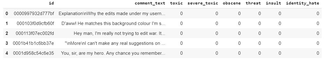
The following script displays the shape of the dataset and it also prints the header of the dataset:
print(toxic_comments.shape)

toxic_comments.head()
Output:
(159571,8)
The dataset contains 159571 records and 8 columns. The header of the dataset looks like this:
Let's remove all the records where any row contains a null value or empty string.
filter = toxic_comments["comment_text"] != ""
toxic_comments = toxic_comments[filter]
toxic_comments = toxic_comments.dropna()
The comment_text column contains text comments. Let's print a random comment and then see the labels for the comments.
print(toxic_comments["comment_text"][168])
Output:
You should be fired, you're a moronic wimp who is too lazy to do research. It makes me sick that people like you exist in this world.
This is clearly a toxic comment. Let's see the associated labels with this comment:
print("Toxic:" + str(toxic_comments["toxic"][168]))
print("Severe_toxic:" + str(toxic_comments["severe_toxic"][168]))
print("Obscene:" + str(toxic_comments["obscene"][168]))
print("Threat:" + str(toxic_comments["threat"][168]))
print("Insult:" + str(toxic_comments["insult"][168]))
print("Identity_hate:" + str(toxic_comments["identity_hate"][168]))
Output:
Toxic:1
Severe_toxic:0
Obscene:0
Threat:0
Insult:1
Identity_hate:0
Let's now plot the comment count for each label. To do so, we will first filter all the label or output columns.
toxic_comments_labels = toxic_comments[["toxic", "severe_toxic", "obscene", "threat", "insult", "identity_hate"]]
toxic_comments_labels.head()
Output:
Using the toxic_comments_labels dataframe, we will plot bar plots that show the total comment counts for different labels.
fig_size = plt.rcParams["figure.figsize"]
fig_size[0] = 10
fig_size[1] = 8
plt.rcParams["figure.figsize"] = fig_size

toxic_comments_labels.sum(axis=0).plot.bar()
Output:
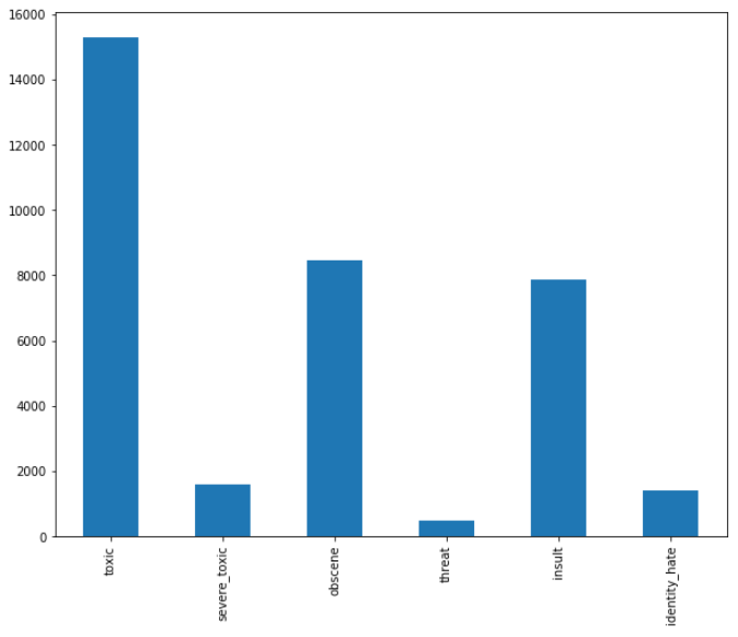
You can see that the "toxic" comment has the highest frequency of occurrence followed by "obscene" and "insult", respectively.
We have successfully analyzed our dataset, in the next section we will create multi-label classification models using this dataset.
Creating Multi-label Text Classification Models
There are two ways to create multi-label classification models: using a single dense output layer and using multiple dense output layers.
In the first approach, we can use a single dense layer with six outputs with sigmoid activation functions and binary cross entropy loss functions. Each neuron in the output dense layer will represent one of the six output labels. The sigmoid activation function will return a value between 0 and 1 for each neuron. If any neuron's output value is greater than 0.5, it is assumed that the comment belongs to the class represented by that particular neuron.
In the second approach we will create one dense output layer for each label. We will have a total of 6 dense layers in the output. Each layer will have its own sigmoid function.
Multi-label Text Classification Model with Single Output Layer
In this section, we will create a multi-label text classification model with a single output layer. As always, the first step in the text classification model is to create a function responsible for cleaning the text.
def preprocess_text(sen):
    # Remove punctuations and numbers
    sentence = re.sub('[^a-zA-Z]', ' ', sen)

    # Single character removal
    sentence = re.sub(r"\s+[a-zA-Z]\s+", ' ', sentence)

    # Removing multiple spaces
    sentence = re.sub(r'\s+', ' ', sentence)

    return sentence
In the next step we will create our input and output set. The input is the comment from the comment_text column. We will clean all the comments and will store them in the X variable. The labels or outputs have already been stored in the toxic_comments_labels dataframe. We will use that dataframe values to store output in the y variable. Look at the following script:
X = []
sentences = list(toxic_comments["comment_text"])
for sen in sentences:
    X.append(preprocess_text(sen))

y = toxic_comments_labels.values
Here we do not need to perform any one-hot encoding because our output labels are already in the form of one-hot encoded vectors.
In the next step, we will divide our data into training and test sets:
X_train, X_test, y_train, y_test = train_test_split(X, y, test_size=0.20, random_state=42)
We need to convert text inputs into embedded vectors. To understand word embeddings in detail, please refer to my article on word embeddings.
tokenizer = Tokenizer(num_words=5000)
tokenizer.fit_on_texts(X_train)

X_train = tokenizer.texts_to_sequences(X_train)
X_test = tokenizer.texts_to_sequences(X_test)

vocab_size = len(tokenizer.word_index) + 1

maxlen = 200

X_train = pad_sequences(X_train, padding='post', maxlen=maxlen)
X_test = pad_sequences(X_test, padding='post', maxlen=maxlen)
We will be using GloVe word embeddings to convert text inputs to their numeric counterparts.
from numpy import array
from numpy import asarray
from numpy import zeros

embeddings_dictionary = dict()

glove_file = open('/content/drive/My Drive/Colab Datasets/glove.6B.100d.txt', encoding="utf8")

for line in glove_file:
    records = line.split()
    word = records[0]
    vector_dimensions = asarray(records[1:], dtype='float32')
    embeddings_dictionary[word] = vector_dimensions
glove_file.close()

embedding_matrix = zeros((vocab_size, 100))
for word, index in tokenizer.word_index.items():
    embedding_vector = embeddings_dictionary.get(word)
    if embedding_vector is not None:
        embedding_matrix[index] = embedding_vector
The following script creates the model. Our model will have one input layer, one embedding layer, one LSTM layer with 128 neurons and one output layer with 6 neurons since we have 6 labels in the output.
deep_inputs = Input(shape=(maxlen,))
embedding_layer = Embedding(vocab_size, 100, weights=[embedding_matrix], trainable=False)(deep_inputs)
LSTM_Layer_1 = LSTM(128)(embedding_layer)
dense_layer_1 = Dense(6, activation='sigmoid')(LSTM_Layer_1)
model = Model(inputs=deep_inputs, outputs=dense_layer_1)

model.compile(loss='binary_crossentropy', optimizer='adam', metrics=['acc'])
Let's print the model summary:
print(model.summary())
Output:
_________________________________________________________________
Layer (type)                 Output Shape              Param #
=================================================================
input_1 (InputLayer)         (None, 200)               0
_________________________________________________________________
embedding_1 (Embedding)      (None, 200, 100)          14824300
_________________________________________________________________
lstm_1 (LSTM)                (None, 128)               117248
_________________________________________________________________
dense_1 (Dense)              (None, 6)                 774
=================================================================
Total params: 14,942,322
Trainable params: 118,022
Non-trainable params: 14,824,300
The following script prints the architecture of our neural network:
from keras.utils import plot_model
plot_model(model, to_file='model_plot4a.png', show_shapes=True, show_layer_names=True)
Output:
Check out our hands-on, practical guide to learning Git, with best-practices, industry-accepted standards, and included cheat sheet. Stop Googling Git commands and actually learn it!
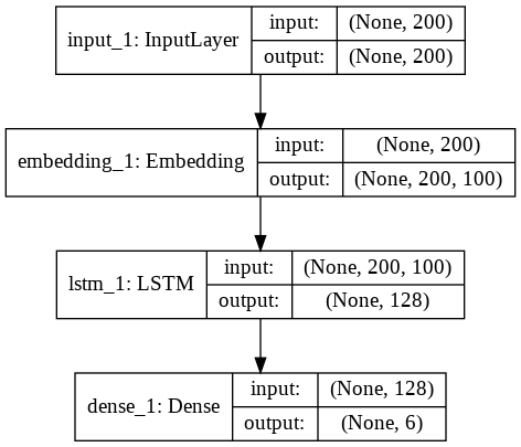
From the figure above, you can see that the output layer only contains 1 dense layer with 6 neurons. Let's now train our model:
history = model.fit(X_train, y_train, batch_size=128, epochs=5, verbose=1, validation_split=0.2)
We will train our model for 5 epochs. You can train the model with more epochs and see if you get better or worse results.
The result for all the 5 epochs is as follows:
rain on 102124 samples, validate on 25532 samples
Epoch 1/5
102124/102124 [==============================] - 245s 2ms/step - loss: 0.1437 - acc: 0.9634 - val_loss: 0.1361 - val_acc: 0.9631
Epoch 2/5
102124/102124 [==============================] - 245s 2ms/step - loss: 0.0763 - acc: 0.9753 - val_loss: 0.0621 - val_acc: 0.9788
Epoch 3/5
102124/102124 [==============================] - 243s 2ms/step - loss: 0.0588 - acc: 0.9800 - val_loss: 0.0578 - val_acc: 0.9802
Epoch 4/5
102124/102124 [==============================] - 246s 2ms/step - loss: 0.0559 - acc: 0.9807 - val_loss: 0.0571 - val_acc: 0.9801
Epoch 5/5
102124/102124 [==============================] - 245s 2ms/step - loss: 0.0528 - acc: 0.9813 - val_loss: 0.0554 - val_acc: 0.9807
Let's now evaluate our model on the test set:
score = model.evaluate(X_test, y_test, verbose=1)

print("Test Score:", score[0])
print("Test Accuracy:", score[1])
Output:
31915/31915 [==============================] - 108s 3ms/step
Test Score: 0.054090796736467786
Test Accuracy: 0.9810642735274182
Our model achieves an accuracy of around 98% which is pretty impressive.
Finally, we will plot the loss and accuracy values for training and test sets to see if our model is overfitting.
import matplotlib.pyplot as plt

plt.plot(history.history['acc'])
plt.plot(history.history['val_acc'])

plt.title('model accuracy')
plt.ylabel('accuracy')
plt.xlabel('epoch')
plt.legend(['train','test'], loc='upper left')
plt.show()

plt.plot(history.history['loss'])
plt.plot(history.history['val_loss'])

plt.title('model loss')
plt.ylabel('loss')
plt.xlabel('epoch')
plt.legend(['train','test'], loc='upper left')
plt.show()
Output:
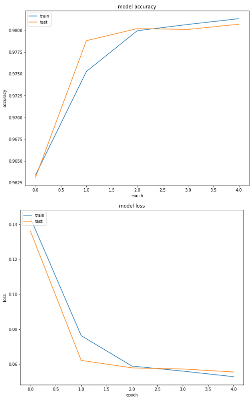
You can see the model is not overfitting on the validation set.
Multi-label Text Classification Model with Multiple Output Layers
In this section we will create a multi-label text classification model where each output label will have a dedicated output dense layer. Let's first define our preprocessing function:
def preprocess_text(sen):
    # Remove punctuations and numbers
    sentence = re.sub('[^a-zA-Z]', ' ', sen)

    # Single character removal
    sentence = re.sub(r"\s+[a-zA-Z]\s+", ' ', sentence)

    # Removing multiple spaces
    sentence = re.sub(r'\s+', ' ', sentence)

    return sentence
The second step is to create inputs and output for the model. The input to the model will be the text comments, whereas the output will be six labels. The following script creates the input layer and the combined output layer:
X = []
sentences = list(toxic_comments["comment_text"])
for sen in sentences:
    X.append(preprocess_text(sen))

y = toxic_comments[["toxic", "severe_toxic", "obscene", "threat", "insult", "identity_hate"]]
Let's divide the data into training and testing sets:
X_train, X_test, y_train, y_test = train_test_split(X, y, test_size=0.20, random_state=42)
The y variable contains the combined output from 6 labels. However, we want to create an individual output layer for each label. We will create 6 variables that store individual labels from the training data and 6 variables that store individual label values for the test data.
Look at the following script:
# First output
y1_train = y_train[["toxic"]].values
y1_test =  y_test[["toxic"]].values

# Second output
y2_train = y_train[["severe_toxic"]].values
y2_test =  y_test[["severe_toxic"]].values

# Third output
y3_train = y_train[["obscene"]].values
y3_test =  y_test[["obscene"]].values

# Fourth output
y4_train = y_train[["threat"]].values
y4_test =  y_test[["threat"]].values

# Fifth output
y5_train = y_train[["insult"]].values
y5_test =  y_test[["insult"]].values

# Sixth output
y6_train = y_train[["identity_hate"]].values
y6_test =  y_test[["identity_hate"]].values
The next step is to convert textual inputs to embedded vectors. The following script does that:
tokenizer = Tokenizer(num_words=5000)
tokenizer.fit_on_texts(X_train)

X_train = tokenizer.texts_to_sequences(X_train)
X_test = tokenizer.texts_to_sequences(X_test)

vocab_size = len(tokenizer.word_index) + 1

maxlen = 200

X_train = pad_sequences(X_train, padding='post', maxlen=maxlen)
X_test = pad_sequences(X_test, padding='post', maxlen=maxlen)
Here again we will use the GloVe word embeddings:
glove_file = open('/content/drive/My Drive/Colab Datasets/glove.6B.100d.txt', encoding="utf8")

for line in glove_file:
    records = line.split()
    word = records[0]
    vector_dimensions = asarray(records[1:], dtype='float32')
    embeddings_dictionary[word] = vector_dimensions
glove_file.close()

embedding_matrix = zeros((vocab_size, 100))
for word, index in tokenizer.word_index.items():
    embedding_vector = embeddings_dictionary.get(word)
    if embedding_vector is not None:
        embedding_matrix[index] = embedding_vector
Now is the time to create our model. Our model will have one input layer, one embedding layer followed by one LSTM layer with 128 neurons. The output from the LSTM layer will be used as the input to the 6 dense output layers. Each output layer will have 1 neuron with sigmoid activation function. Each output will predict integer value between 1 and 0 for the corresponding label.
The following script creates our model:
input_1 = Input(shape=(maxlen,))
embedding_layer = Embedding(vocab_size, 100, weights=[embedding_matrix], trainable=False)(input_1)
LSTM_Layer1 = LSTM(128)(embedding_layer)

output1 = Dense(1, activation='sigmoid')(LSTM_Layer1)
output2 = Dense(1, activation='sigmoid')(LSTM_Layer1)
output3 = Dense(1, activation='sigmoid')(LSTM_Layer1)
output4 = Dense(1, activation='sigmoid')(LSTM_Layer1)
output5 = Dense(1, activation='sigmoid')(LSTM_Layer1)
output6 = Dense(1, activation='sigmoid')(LSTM_Layer1)

model = Model(inputs=input_1, outputs=[output1, output2, output3, output4, output5, output6])
model.compile(loss='binary_crossentropy', optimizer='adam', metrics=['acc'])
The following script prints the summary of the model:
print(model.summary())
Output:
__________________________________________________________________________________________________
Layer (type)                    Output Shape         Param #     Connected to
==================================================================================================
input_1 (InputLayer)            (None, 200)          0
__________________________________________________________________________________________________
embedding_1 (Embedding)         (None, 200, 100)     14824300    input_1[0][0]
__________________________________________________________________________________________________
lstm_1 (LSTM)                   (None, 128)          117248      embedding_1[0][0]
__________________________________________________________________________________________________
dense_1 (Dense)                 (None, 1)            129         lstm_1[0][0]
__________________________________________________________________________________________________
dense_2 (Dense)                 (None, 1)            129         lstm_1[0][0]
__________________________________________________________________________________________________
dense_3 (Dense)                 (None, 1)            129         lstm_1[0][0]
__________________________________________________________________________________________________
dense_4 (Dense)                 (None, 1)            129         lstm_1[0][0]
__________________________________________________________________________________________________
dense_5 (Dense)                 (None, 1)            129         lstm_1[0][0]
__________________________________________________________________________________________________
dense_6 (Dense)                 (None, 1)            129         lstm_1[0][0]
==================================================================================================
Total params: 14,942,322
Trainable params: 118,022
Non-trainable params: 14,824,300
And the following script prints the architecture of our model:
from keras.utils import plot_model
plot_model(model, to_file='model_plot4b.png', show_shapes=True, show_layer_names=True)
Output:
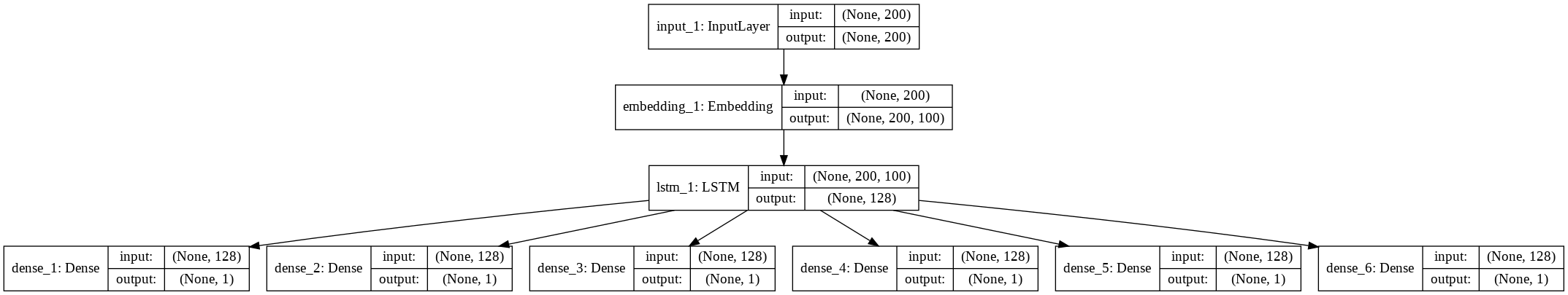
You can see that we have 6 different output layers. The above figure clearly explains the difference between the model with a single input layer that we created in the last section and the model with multiple output layers.
Let's now train our model:
history = model.fit(x=X_train, y=[y1_train, y2_train, y3_train, y4_train, y5_train, y6_train], batch_size=8192, epochs=5, verbose=1, validation_split=0.2)
I tried to run the model for five epochs but it was terribly overfitting on the validation set. I increased the batch size but still the test accuracy was not so good. One of the possible reasons for overfitting is that here in this case we have an individual output layer for each label which increases the complexity of our model. The increase in model complexity often leads to overfitting.
The result for each epoch is shown below:
Output:
Train on 102124 samples, validate on 25532 samples
Epoch 1/5
102124/102124 [==============================] - 24s 239us/step - loss: 3.5116 - dense_1_loss: 0.6017 - dense_2_loss: 0.5806 - dense_3_loss: 0.6150 - dense_4_loss: 0.5585 - dense_5_loss: 0.5828 - dense_6_loss: 0.5730 - dense_1_acc: 0.9029 - dense_2_acc: 0.9842 - dense_3_acc: 0.9444 - dense_4_acc: 0.9934 - dense_5_acc: 0.9508 - dense_6_acc: 0.9870 - val_loss: 1.0369 - val_dense_1_loss: 0.3290 - val_dense_2_loss: 0.0983 - val_dense_3_loss: 0.2571 - val_dense_4_loss: 0.0595 - val_dense_5_loss: 0.1972 - val_dense_6_loss: 0.0959 - val_dense_1_acc: 0.9037 - val_dense_2_acc: 0.9901 - val_dense_3_acc: 0.9469 - val_dense_4_acc: 0.9966 - val_dense_5_acc: 0.9509 - val_dense_6_acc: 0.9901
Epoch 2/5
102124/102124 [==============================] - 20s 197us/step - loss: 0.9084 - dense_1_loss: 0.3324 - dense_2_loss: 0.0679 - dense_3_loss: 0.2172 - dense_4_loss: 0.0338 - dense_5_loss: 0.1983 - dense_6_loss: 0.0589 - dense_1_acc: 0.9043 - dense_2_acc: 0.9899 - dense_3_acc: 0.9474 - dense_4_acc: 0.9968 - dense_5_acc: 0.9510 - dense_6_acc: 0.9915 - val_loss: 0.8616 - val_dense_1_loss: 0.3164 - val_dense_2_loss: 0.0555 - val_dense_3_loss: 0.2127 - val_dense_4_loss: 0.0235 - val_dense_5_loss: 0.1981 - val_dense_6_loss: 0.0554 - val_dense_1_acc: 0.9038 - val_dense_2_acc: 0.9900 - val_dense_3_acc: 0.9469 - val_dense_4_acc: 0.9965 - val_dense_5_acc: 0.9509 - val_dense_6_acc: 0.9900
Epoch 3/5
102124/102124 [==============================] - 20s 199us/step - loss: 0.8513 - dense_1_loss: 0.3179 - dense_2_loss: 0.0566 - dense_3_loss: 0.2103 - dense_4_loss: 0.0216 - dense_5_loss: 0.1960 - dense_6_loss: 0.0490 - dense_1_acc: 0.9043 - dense_2_acc: 0.9899 - dense_3_acc: 0.9474 - dense_4_acc: 0.9968 - dense_5_acc: 0.9510 - dense_6_acc: 0.9915 - val_loss: 0.8552 - val_dense_1_loss: 0.3158 - val_dense_2_loss: 0.0566 - val_dense_3_loss: 0.2074 - val_dense_4_loss: 0.0225 - val_dense_5_loss: 0.1960 - val_dense_6_loss: 0.0568 - val_dense_1_acc: 0.9038 - val_dense_2_acc: 0.9900 - val_dense_3_acc: 0.9469 - val_dense_4_acc: 0.9965 - val_dense_5_acc: 0.9509 - val_dense_6_acc: 0.9900
Epoch 4/5
102124/102124 [==============================] - 20s 198us/step - loss: 0.8442 - dense_1_loss: 0.3153 - dense_2_loss: 0.0570 - dense_3_loss: 0.2061 - dense_4_loss: 0.0213 - dense_5_loss: 0.1952 - dense_6_loss: 0.0493 - dense_1_acc: 0.9043 - dense_2_acc: 0.9899 - dense_3_acc: 0.9474 - dense_4_acc: 0.9968 - dense_5_acc: 0.9510 - dense_6_acc: 0.9915 - val_loss: 0.8527 - val_dense_1_loss: 0.3156 - val_dense_2_loss: 0.0558 - val_dense_3_loss: 0.2074 - val_dense_4_loss: 0.0226 - val_dense_5_loss: 0.1951 - val_dense_6_loss: 0.0561 - val_dense_1_acc: 0.9038 - val_dense_2_acc: 0.9900 - val_dense_3_acc: 0.9469 - val_dense_4_acc: 0.9965 - val_dense_5_acc: 0.9509 - val_dense_6_acc: 0.9900
Epoch 5/5
102124/102124 [==============================] - 20s 197us/step - loss: 0.8410 - dense_1_loss: 0.3146 - dense_2_loss: 0.0561 - dense_3_loss: 0.2055 - dense_4_loss: 0.0213 - dense_5_loss: 0.1948 - dense_6_loss: 0.0486 - dense_1_acc: 0.9043 - dense_2_acc: 0.9899 - dense_3_acc: 0.9474 - dense_4_acc: 0.9968 - dense_5_acc: 0.9510 - dense_6_acc: 0.9915 - val_loss: 0.8501 - val_dense_1_loss: 0.3153 - val_dense_2_loss: 0.0553 - val_dense_3_loss: 0.2069 - val_dense_4_loss: 0.0226 - val_dense_5_loss: 0.1948 - val_dense_6_loss: 0.0553 - val_dense_1_acc: 0.9038 - val_dense_2_acc: 0.9900 - val_dense_3_acc: 0.9469 - val_dense_4_acc: 0.9965 - val_dense_5_acc: 0.9509 - val_dense_6_acc: 0.9900
You can see that for each epoch, we have values for loss, value loss, accuracy, and value accuracy for all the 6 dense layers in the output.
Let's now evaluate the performance of our model on the test set:
score = model.evaluate(x=X_test, y=[y1_test, y2_test, y3_test, y4_test, y5_test, y6_test], verbose=1)

print("Test Score:", score[0])
print("Test Accuracy:", score[1])
Output:
31915/31915 [==============================] - 111s 3ms/step
Test Score: 0.8471985269747015
Test Accuracy: 0.31425264998511726
An accuracy of only 31% is achieved on the test set via multiple output layers.
The following script plots the loss and accuracy values for training and validation sets for the first dense layer.
import matplotlib.pyplot as plt

plt.plot(history.history['dense_1_acc'])
plt.plot(history.history['val_dense_1_acc'])

plt.title('model accuracy')
plt.ylabel('accuracy')
plt.xlabel('epoch')
plt.legend(['train','test'], loc='upper left')
plt.show()

plt.plot(history.history['dense_1_loss'])
plt.plot(history.history['val_dense_1_loss'])

plt.title('model loss')
plt.ylabel('loss')
plt.xlabel('epoch')
plt.legend(['train','test'], loc='upper left')
plt.show()
Output:
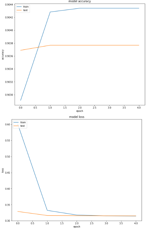
From the output you can see that the accuracy for the test (validation) set doesn't converge after the first epochs. Also, the difference between training and validation accuracy is very minimal. Therefore, the model starts to overfit after the first epochs and hence we get poor performance on unseen test sets.
Conclusion
Multi-label text classification is one of the most common text classification problems. In this article, we studied two deep learning approaches for multi-label text classification. In the first approach we used a single dense output layer with multiple neurons where each neuron represented one label.
In the second approach, we created separate dense layers for each label with one neuron. Results show that in our case, a single output layer with multiple neurons works better than multiple output layers.
As a next step, I would advise you to change the activation function and the train test split to see if you can get better results than the one presented in this article.

