Python with Pandas: DataFrame Tutorial with Examples

Introduction

Pandas is an open-source Python library for data analysis. It is designed for efficient and intuitive handling and processing of structured data.

The two main data structures in Pandas are Series and DataFrame. Series are essentially one-dimensional labeled arrays of any type of data, while DataFrames are two-dimensional, with potentially heterogeneous data types, labeled arrays of any type of data. Heterogeneous means that not all "rows" need to be of equal size.

In this article we will go through the most common ways of creating a DataFrame and methods to change their structure.

We'll be using the Jupyter Notebook since it offers a nice visual representation of DataFrames. Though, any IDE will also do the job, just by calling a print() statement on the DataFrame object.

Creating DataFrames

Whenever you create a DataFrame, whether you're creating one manually or generating one from a data source such as a file - the data has to be ordered in a tabular fashion, as a sequence of rows containing data.

This implies that the rows share the same order of fields, i.e. if you want to have a DataFrame with information about a person's name and age, you want to make sure that all your rows hold the information in the same way.

Any discrepancy will cause the DataFrame to be faulty, resulting in errors.

Creating an Empty DataFrame

To create an empty DataFrame is as simple as:

import pandas as pd
dataFrame1 = pd.DataFrame()

We will take a look at how you can add rows and columns to this empty DataFrame while manipulating their structure.

Creating a DataFrame From Lists

Following the "sequence of rows with the same order of fields" principle, you can create a DataFrame from a list that contains such a sequence, or from multiple lists zip()-ed together in such a way that they provide a sequence like that:

import pandas as pd

listPepper = [ 
            [50, "Bell pepper", "Not even spicy"], 
            [5000, "Espelette pepper", "Uncomfortable"], 
            [500000, "Chocolate habanero", "Practically ate pepper spray"]
            ]

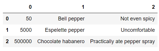
dataFrame1 = pd.DataFrame(listPepper)

dataFrame1
# If you aren't using Jupyter, you'll have to call `print()`
# print(dataFrame1) 

This results in:

The same effect could have been achieved by having the data in multiple lists and zip()-ing them together. This approach can be used when the data we have is provided with lists of values for a single column (field), instead of the aforementioned way in which a list contains data for each particular row as a unit.

Meaning that we have all the data (in order) for columns individually, which, when zipped together, create rows.

You may have noticed that the column and row labels aren't very informative in the DataFrame we've created. You can pass additional information when creating the DataFrame, and one thing you can do is give the row/column labels you want to use:

import pandas as pd

listScoville = [50, 5000, 500000]
listName = ["Bell pepper", "Espelette pepper", "Chocolate habanero"]
listFeeling = ["Not even spicy", "Uncomfortable", "Practically ate pepper spray"]

dataFrame1 = pd.DataFrame(zip(listScoville, listName, listFeeling), columns = ['Scoville', 'Name', 'Feeling'])

# Print the dataframe
dataFrame1

Which would give us the same output as before, just with more meaningful column names:

Another data representation you can use here is to provide the data as a list of dictionaries in the following format:

listPepper = [
    { columnName1 : valueForRow1, columnName2: valueForRow1, ... },
    { columnName1 : valueForRow2, columnName2: valueForRow2, ... },
    ...
]

In our example the representation would look like this:

listPepper = [
  {'Scoville' : 50, 'Name' : 'Bell pepper', 'Feeling' : 'Not even spicy'},
  {'Scoville' : 5000, 'Name' : 'Espelette pepper', 'Feeling' : 'Uncomfortable'},
  {'Scoville' : 500000, 'Name' : 'Chocolate habanero', 'Feeling' : 'Practically ate pepper spray'},
]

And we would create the DataFrame in the same way as before:

dataFrame1 = pd.DataFrame(listPepper)

Creating a DataFrame From Dictionaries

Dictionaries are another way of providing data in the column-wise fashion. Every column is given a list of values rows contain for it, in order:

dictionaryData = {
    'columnName1' : [valueForRow1, valueForRow2, valueForRow3...],
    'columnName2' : [valueForRow1, valueForRow2, valueForRow3...],
    ....
}

Let's represent the same data as before, but using the dictionary format:

import pandas as pd
dictionaryData = {
    'Scoville' : [50, 5000, 500000],
    'Name' : ["Bell pepper", "Espelette pepper", "Chocolate habanero"],
    'Feeling' : ["Not even spicy", "Uncomfortable", "Practically ate pepper spray"]
}

dataFrame1 = pd.DataFrame(dictionaryData)

# Print the dataframe
dataFrame1

Which gives us the expected output:

Reading a DataFrame From a File

There are many file types supported for reading and writing DataFrames. Each respective filetype function follows the same syntax read_filetype(), such as read_csv(), read_excel(), read_json(), read_html(), etc...

A very common file type is .csv (Comma-Separated-Values). The rows are provided as lines, with the values they are supposed to contain separated by a delimiter (most often a comma). You can set another delimiter via the sep argument.

If you aren't familiar with the .csv file type, this is an example of what it looks like:

Scoville, Name, Feeling
50, Bell pepper, Not even spicy 
5.000, Espelette pepper, Uncomfortable
10.000, Serrano pepper, I regret this
60.000, Bird's eye chili, 4th stage of grief 
500.000, Chocolate habanero, Practically ate pepper spray
2.000.000, Carolina Reaper, Actually ate pepper spray

Note that the first line in the file are the column names. You can of course specify from which line Pandas should start reading the data, but, by default Pandas treats the first line as the column names and starts loading the data in from the second line:

import pandas as pd

pepperDataFrame = pd.read_csv('pepper_example.csv')

# For other separators, provide the `sep` argument
# pepperDataFrame = pd.read_csv('pepper_example.csv', sep=';')

pepperDataFrame
#print(pepperDataFrame)

Which gives us the output:

Manipulating DataFrames

This section will be covering the basic methods for changing a DataFrame's structure. However, before we get into that topic you should know how to access individual rows or groups of rows, as well as columns.

Accessing/Locating Elements

Pandas has two different ways of selecting data - loc[] and iloc[].

loc[] allows you to select rows and columns by using labels, like row['Value'] and column['Other Value']. Meanwhile, iloc[] requires that you pass in the index of the entries you want to select, so you can only use numbers. You may also select columns just by passing in their name in brackets. Let’s see how this works in action:

# Location by label
# Here, '5' is treated as the *label* of the index, not its value
print(pepperDataFrame.loc[5])
# Location by index
print(pepperDataFrame.iloc[1]) 

Output:

Scoville               2.000.000
 Name                  Carolina Reaper
 Feeling               Actually ate pepper spray
Name: 5, dtype: object
Scoville               5.000
 Name                  Espelette pepper
 Feeling               Uncomfortable
Name: 1, dtype: object

This also works for a group of rows, such as from 0...n:

print(pepperDataFrame.loc[:1]) 

This outputs:

It's important to note that iloc[] always expects an integer. loc[] supports other data types as well. We can use an integer here too, though we can also use other data types such as strings.

You can also access specific values for elements. For example, we might want to access the element in the 2nd row, though only return its Name value:

print(pepperDataFrame.loc[2, 'Name'])

This returns:

Chocolate habanero

Accessing columns is as simple as writing dataFrameName.ColumnName or dataFrameName['ColumnName']. The second option is preferred since the column can have the same name as a predefined Pandas method, and using the first option in that case could cause bugs:

print(pepperDataFrame['Name']) 
# Same output as print(pepperDataFrame.Name)

This outputs:

0           Bell pepper
1      Espelette pepper
2    Chocolate habanero
Name: Name, dtype: object

Columns can also be accessed by using loc[] and iloc[]. For example, we'll access all rows, from 0...n where n is the number of rows and fetch the first column. This has the same output as the previous line of code:

dataFrame1.iloc[:, 1] # or dataFrame1.loc[:, 'Name']

Manipulating Indices

Indices are row labels in a DataFrame, and they are what we use when we want to access rows. Since we didn't change the default indices Pandas assigned to DataFrames upon their creation, all our rows have been labeled with integers from 0 and up.

The first way we can change the indexing of our DataFrame is by using the set_index() method. We pass any of the columns in our DataFrame to this method and it becomes the new index. So we can either create indices ourselves or simply assign a column as the index.

Note that the method doesn't change the original DataFrame but instead returns a new DataFrame with the new index, so we have to assign the return value to the DataFrame variable if we want to keep the change, or set the inplace flag to True:

import pandas as pd

listPepper = [
  {'Scoville' : 50, 'Name' : 'Bell pepper', 'Feeling' : 'Not even spicy'},
  {'Scoville' : 5000, 'Name' : 'Espelette pepper', 'Feeling' : 'Uncomfortable'},
  {'Scoville' : 500000, 'Name' : 'Chocolate habanero', 'Feeling' : 'Practically ate pepper spray'},
]

dataFrame1 = pd.DataFrame(listPepper)
dataFrame2 = dataFrame1.set_index('Scoville')

dataFrame2

Output:

This would work just as well:

dataFrame1 = pd.DataFrame(listPepper)
dataFrame1.set_index('Scoville', inplace=True)

dataFrame1

Now that we have a non-default index we can use a new set of values, using reindex(), Pandas will automatically fill the values with NaN for every index that can't be matched with an existing row:

new_index = [50, 5000, 'New value not present in the data frame']
dataFrame1.reindex(new_index)

Output:

You can control what value Pandas uses to fill in the missing values by setting the optional parameter fill_value:

dataFrame1.reindex(new_index, fill_value=0)

Output:

Since we have set a new index for our DataFrame, loc[] now works with that index:

dataFrame1.loc[5000] 
# dataFrame1.iloc[5000] outputs the same in this case

This results in:

Name       Espelette pepper
Feeling       Uncomfortable
Name: 5000, dtype: object

Manipulating Rows

Adding and removing rows becomes simple if you're comfortable with using loc[]. If you set a row that doesn't exist, it's created:

dataFrame1.loc[50] = [10000, 'Serrano pepper', 'I regret this']
dataFrame1

Output:

And if you want to remove a row, you specify its index to the drop() function. It takes an optional parameter, axis. The axis accepts 0/index or 1/columns. Depending on this, the drop() function either drops the row it's called upon, or the column it's called upon.

Not specifying a value for the axis parameter will delete the corresponding row by default, as axis is 0 by default:

dataFrame1.drop(1, inplace=True) 
# Same as dataFrame1.drop(1, axis=0)

Output:

You can also rename rows that already exist in the table. The rename() function accepts a dictionary of changes you wish to make:

dataFrame1.rename({0:"First", 1:"Second"}, inplace=True)

Output:

Note that drop() and rename() also accept the optional parameter - inplace. Setting this to True (False by default) will tell Pandas to change the original DataFrame instead of returning a new one. If left unset, you'll have to pack the resulting DataFrame into a new one to persist the changes.

Another useful method you should be aware of is the drop_duplicates() function which removes all duplicate rows from the DataFrame. Let's demonstrate this by adding two duplicate rows:

dataFrame1.loc[3] = [60.000, "Bird's eye chili", "4th stage of grief"]
dataFrame1.loc[4] = [60.000, "Bird's eye chili", "4th stage of grief"]

dataFrame1

Which gives us the output:

Now we can call drop_duplicates():

dataFrame1.drop_duplicates(inplace=True)

dataFrame1

And the duplicate rows will be removed:

Manipulating Columns

New columns can be added in a similar way to adding rows:

dataFrame1['Color'] = ['Green', 'Bright Red', 'Brown']
dataFrame1

Output:

Also similarly to rows, columns can be removed by calling the drop() function, the only difference being that you have to set the optional parameter axis to 1 so that Pandas knows you want to remove a column and not a row:

dataFrame1.drop('Feeling', axis=1, inplace=True)

Output:

When it comes to renaming columns, the rename() function needs to be told specifically that we mean to change the columns by setting the optional parameter columns to the value of our "change dictionary":

dataFrame1.rename(columns={"Feeling":"Measure of Pain"}, inplace=True)

Output:

Again, same as with removing/renaming rows, you can set the optional parameter inplace to True if you want the original DataFrame modified instead of the function returning a new DataFrame.

Conclusion

In this article, we've gone over what Pandas DataFrames are, as they're a key class from the Pandas framework used to store data.

We've learned how to create a DataFrame manually, using a list and dictionary, after which we've read data from a file.

Then, we've manipulated the data in the DataFrame - using loc[] and iloc[], we've located data, created new rows and columns, renamed existing ones and then dropped them.