Simulated Annealing Optimization Algorithm in Java

Introduction

Simulated Annealing is an evolutionary algorithm inspired by annealing from metallurgy. It's a closely controlled process where a metallic material is heated above its recrystallization temperature and slowly cooled.

Successful annealing has the effect of lowering the hardness and thermodynamic free energy of the metal and altering its internal structure such that the crystal structures inside the material become deformation-free. The end result is a piece of metal with increased elasticity and less deformations which makes the material more workable.

This process serves as a direct inspiration for yet another optimization algorithm. We simulate the annealing process in a search space to find an approximate global optimum. The slow cooling in this algorithm is translated as a lower probability to accept a worse solution than the current solution as the search space is slowly explored.

That being said, Simulated Annealing is a probabilistic meta-heuristic used to find an approximately good solution and is typically used with discrete search spaces.

In this article, we'll be using it on a discrete search space - on the Traveling Salesman Problem.

Simulated Annealing

Mathematical Model

The key concept in simulated annealing is energy. We have already mentioned that the process of annealing leads to a material with a lower energy state. This lower energy state is the result of a slow process of cooling the material from a high temperature (i.e. high energy level) towards lower temperature (i.e. low energy level).

For a given material, we can define two energy states, E₁ (current state) and E₂ (next state), and their difference:

$$
\Delta E = E_2-E_1
$$

In general, the process of annealing will result in transitions from higher to lower energy states, i.e. where ΔE < 0. Such transitions always occur with the probability 1 since they are in our interest for finding the best possible solutions.

Sometimes during the process, however, the energy is unable to keep decreasing in a monotonic way due to some specifics of the material's inner structure. In such cases, an increase in energy is necessary before the material can continue decreasing its energy.

If ΔE > 0 , the energy level of the next state is higher than the energy level of the current state. In this case, the probability of jumping from state E₁ into a higher-energy state E₂ is determined by the probability:

$$
P(\Delta E) = exp({\frac{-\Delta E}{k \cdot T}})
$$

Where k represents the Boltzmann constant and T is the current temperature of the material. By changing the temperature of the material, we see that the energy level of the material changes as well.

Simulating the Annealing Model

To simulate the process of annealing, we start in some initial state, which is randomly determined at the beginning of the algorithm. From this point, we wish to reach the optimal state, typically a minimum or a maximum value. Both the initial and the optimal states (along all other states) exist within our search space which is characterized by the problem we are trying to solve.

The analogy of the previously described energy model in the context of simulated annealing is that we are trying to minimize a certain target function which characterizes our optimization problem. This function essentially represents the energy level of the material which we are trying to minimize. Therefore, the idea of minimizing energy levels boils down to minimizing the target function of our optimization problem.

Let's see a very simple example of an optimization problem. In case our problem is finding the minimum of a quadratic function, the function itself represents the search space and each of the points (e.g. (x=1;y=-2)), represents one of the states:

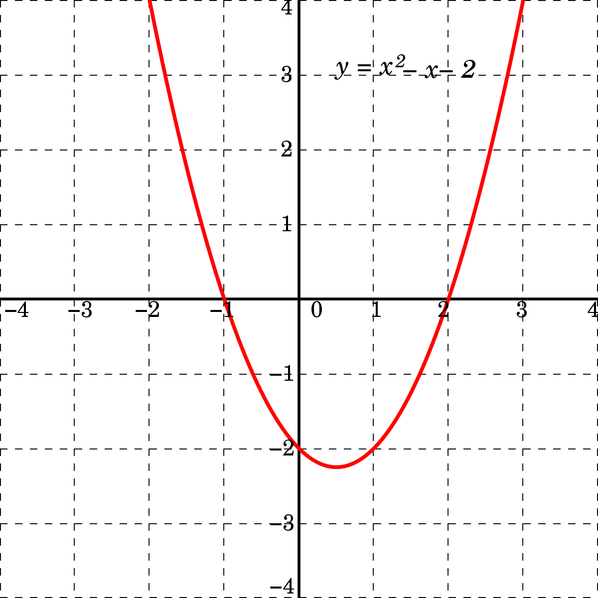
Credit: Wikipedia

To make finding new solutions possible, we must accept them according to some predefined rules. In the example above, we would prefer $x=1$ over $x=2$ since it would lead us closer to the minimum.

In some cases, however, we might want to allow the algorithm to accept worse solutions to avoid potential local optimums.

To allow the algorithm to accept new solutions which are either better, or seemingly worse but will help us avoid local optimums, we can use the previously defined probabilities of the simulated annealing algorithm: in case our new solution is better than our current solution, we will always accept it.

In case the new solution is worse, we will accept it with some probability:

$$
P = exp({-\frac{f(s_2)-f(s_1)}{T_k}})
$$

where s is some solution and Tk is the temperature in the k-th step of the algorithm.

Notice how this expression is analogous to the previous one describing the annealing process with energy levels. The difference is that here, instead of energy levels, we have function values.

Also, by slowly decreasing the temperature during the duration of the algorithm, we are decreasing the probability of accepting worse solutions. In early stages, this acceptance of worse solutions could help us immensely because it allows the algorithm to look for solutions in a vast solution space and jump out of a local optimum if it encounters any.

By decreasing the temperature (and thus the probability of accepting worse solutions) we are allowing the algorithm to slowly focus on a specific area which ideally contains the optimal solution. This slow cooling process is what makes the algorithm quite effective when dealing with local optimums.

Here's a great visualization of how the search space is being analyzed:

Credit: Wikipedia

Motivation

Now that we have covered the inner workings of the algorithm, let's see a motivational example which we will follow in the rest of this article.

One of the most famous optimization problems is the Traveling Salesman Problem. Here we have a set of points (cities) which we want to traverse in such a way to minimize the total travel distance.

This can be represented as a function since we would have a different total distance depending on the order in which we traverse the cities:

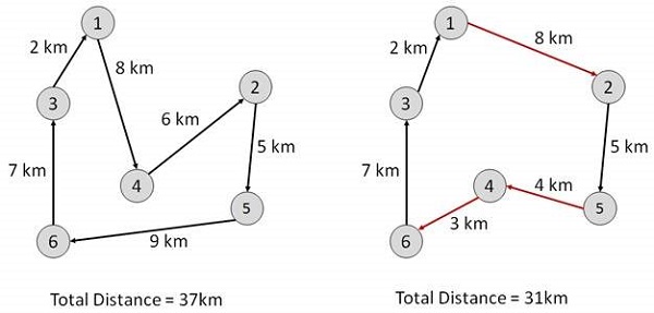
Credit: TutorialsPoint

Two different tours for the same layout of cities. The function in this case represents the total distance traveled.

Now if we do some simple math, we will deduce that the total number of combinations for traversing all cities is N!, where N is the number of cities. For example, if we have three cities, there would be six possible combinations:

1 -> 2 -> 3
1 -> 3 -> 2
2 -> 1 -> 3
2 -> 3 -> 1
3 -> 1 -> 2
3 -> 2 -> 1

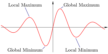
One of these combinations would categorically have the shortest distance and one of them would have the longest.

These two values would then represent our global optimums, i.e. global minimum and global maximum. Since we wish to find the shortest total distance, we opt for finding the global minimum:

Implementation

To start solving the Traveling Salesman Problem (TSP), we first need to create some initial data structures. For TSP, this means creating helper classes City, Tour, and Util.

Helper Classes

The City class is quite simple. It represents a city in two-dimensional space with the x and y coordinates it receives through the constructor.

public class City {

    private int x;
    private int y;

    public City(int x, int y) {
        this.x = x;
        this.y = y;
    }

    // Getters and toString()
}

The Tour class is slightly more complex but the only "real" logic here happens in the getTourLength() method. We start from the first city in our tour and begin traversing the list. We calculate the distance between each pair of neighboring cities and add it to the total distance.

At the end of the method, we have computed the total distance of our tour:

public class Tour {
    private List<City> cities;
    private int distance;

    public Tour(List<City> cities) {
        this.cities = new ArrayList<>(cities);
        Collections.shuffle(this.cities);
    }
    public City getCity(int index) {
        return cities.get(index);
    }

    public int getTourLength() {
        if (distance != 0) return distance;

        int totalDistance = 0;

        for (int i = 0; i < noCities(); i++) {
            City start = getCity(i);
            City end = getCity(i + 1 < noCities() ? i + 1 : 0);
            totalDistance += Util.distance(start, end);
        }

        distance = totalDistance;
        return totalDistance;
    }

    public Tour duplicate() {
        return new Tour(new ArrayList<>(cities));
    }

    public int noCities() {
        return cities.size();
    }

    // Getters and toString()
}

The final helper class that needs to be mentioned is the Util class which contains the probability() and distance() methods:

public class Util {
    public static double probability(double f1, double f2, double temp) {
        if (f2 < f1) return 1;
        return Math.exp((f1 - f2) / temp);
    }

    public static double distance(City city1, City city2) {
        int xDist = Math.abs(city1.getX() - city2.getX());
        int yDist = Math.abs(city1.getY() - city2.getY());
        return Math.sqrt(xDist * xDist + yDist * yDist);
    }
}

The first method is essentially the implementation of our mathematical model mentioned earlier. If the length of the second tour is shorter than the length of the first tour, we will keep the first tour. Otherwise, we'll return the probability of accepting the second tour.

The distance() method computes and returns the Euclidean distance between the two given cities.

Implementing Simulated Annealing

With our helpers out of the way, let's go ahead and implement the algorithm itself:

public class SimulatedAnnealing {
    private static double temperature = 1000;
    private static double coolingFactor = 0.995;

    public static void main(String[] args) {
        List<City> cities = new ArrayList<>();

        City city1 = new City(100, 100);
        cities.add(city1);

        City city2 = new City(200, 200);
        cities.add(city2);

        City city3 = new City(100, 200);
        cities.add(city3);

        City city4 = new City(200, 100);
        cities.add(city4);

        Tour current = new Tour(cities);
        Tour best = current.duplicate();

        for (double t = temperature; t > 1; t *= coolingFactor) {
            Tour neighbor = current.duplicate();

            int index1 = (int) (neighbor.noCities() * Math.random());
            int index2 = (int) (neighbor.noCities() * Math.random());

            Collections.swap(next.getCities(), index1, index2);

            int currentLength = current.getTourLength();
            int neighborLength = neighbor.getTourLength();

            if (Math.random() < Util.probability(currentLength, neighborLength, t)) {
                current = neighbor.duplicate();
            }

            if (current.getTourLength() < best.getTourLength()) {
                best = current.duplicate();
            }
        }

        System.out.println("Final tour length: " + best.getTourLength());
        System.out.println("Tour: " + best);
    }
}

We start by adding some cities to a list. For simplicity, we added four cities representing a square. We then create a new tour and start going through the main loop, slowly lowering the temperature by a cooling factor.

In each iteration of the loop, we generate a neighboring solution by randomly swapping two cities in our current tour. By using the probability method, the algorithm determines whether the neighboring solution will be accepted or not.

When the algorithm is just starting, the high temperature will cause the acceptance probability to be higher, making it more likely to accept the neighbor as our next solution. As the temperature slowly decreases, so does the probability.

This will have the effect of initially jumping through various permutations of possible tours (even bad ones) because they might be able to lead us to a more optimal solution in the future.

The final output of the program is shown below:

Final tour length: 400
Tour: [(100, 100), (200, 100), (200, 200), (100, 200)]

The best tour found by the algorithm is the one starting from the bottom left corner and then going counter-clockwise. This gives the minimum tour length of 400.

Conclusion

Simulated Annealing is a very appealing algorithm because it takes inspiration from a real-world process. As other Evolutionary Algorithms, it has the potential to solve some difficult problems.

However, no algorithm is perfect and ideal for any kind of problem (see No Free Lunch Theorem). This means that we must be clever when choosing which algorithm to use and when. Sometimes, the answer is obvious. But sometimes, it takes time and effort to really figure out which techniques give the best possible results in practice.