What's New in Tensorflow 2.0?

Introduction

If you are a Machine Learning Engineer, Data Scientist, or a hobbyist developing Machine Learning Models from time to time just for fun, then it is very likely that you are familiar with Tensorflow.

Tensorflow is an open-source and free framework developed by Google Brain Team written in Python, C++, and CUDA. It is used to develop, test, and deploy Machine Learning models.

Initially, TensorFlow did not have full support for multiple platforms and programming languages, and it was not very fast and efficient for training Machine Learning models, but with time and after a few updates, Tensorflow is now considered as a go-to framework for developing, training and deploying machine learning models.

TensorFlow 1.x

Tensorflow 1.x was also a huge leap for this framework. It introduced many new features, improved performance, and open source contributions. It introduced a high-level API for TensorFlow, which made it very easy to build prototypes in no time.

It was made compatible with Keras. But the major thing that irritated the developers was that it did not feel like taking advantage of the simplicity of Python when using TensorFlow.

In TensorFlow, every model is represented as a graph, and the nodes represent the computations in the graph. It is an example of "Symbolic Programming" and whereas Python is an "Imperative Programming" Language.

I will not go into much detail as this is beyond the scope of this article. But the point here is that with the release of PyTorch (which is much oriented towards Imperative Programming and takes advantage of Python's dynamic behavior), newbies and research scientists found PyTorch easier to understand and learn than Tensorflow and in no time PyTorch started to gain popularity.

Every Tensorflow developer was demanding the same from Tensorflow and the Google Brain Team. Moreover, TensorFlow 1.x went through a lot of development which resulted in many APIs, i.e., tf.layers, tf.contrib.layers, tf.keras and the developers had many options to choose from, which resulted in conflicts.

Announcement of Tensorflow 2.0

It was pretty obvious that the Tensorflow team had to address these issues so they announced Tensorflow 2.0.

This was a huge step because to address all the issues they had to make huge changes. Many people were faced with another learning experience, but the improvements made it worth relearning.

In the training phase, we're introduced to tf.data and Datasets, which allow us to import and process data with ease. Then, we're introduced to distributed training over multiple CPUs, GPUs and TPUs. For serialization, we can use the SavedModel to either deploy to TensorFlow Hub or services like TensorFlow Serving, TensorFlow Lite or TensorFlow.js:

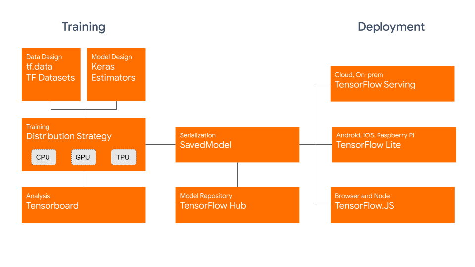
Credit: blog.tensorflow.org

What's new in Tensorflow 2.0

Here is a brief overview of the most important updates that came with Tensorflow 2.

1. Deploying Models on Multiple Platforms

Tensorflow was always very well suited for production, but Tensorflow 2 improved compatibility and parity across multiple platforms.

It introduced the new platform support for the SavedModel format that allows us to save Tensorflow models. The novelty here is that you can deploy your saved model on any platform, i.e., on Mobile or IoT devices using Tensorflow Lite or Node.js with Tensorflow.js. Alternatively, you can use it in production environments with Tensorflow Serving.

Let's take a look at how you can save a compiled model:

import os
import tensorflow as tf
# Building the Model
model = tf.keras.Sequential([
        tf.keras.layers.Dense(5,actiavtion='relu',input_shape=(16,)),
        tf.keras.layers.Dense(1,activation='sigmoid')])
# Compiling the Model
model.compile(loss='binary_crossentropy',optimizer='adam')

# Saving the Model
save_path = path + "/version_number/"
save_path = os.path.join
tf.saved_model.save(model, save_path)

And there you go. You can now deploy it using any of the aforementioned services.

2. Eager Execution

Before Tensorflow 2, you had to create a session to run your model. In fact, if you wanted to print the value of a variable just for debugging, you first had to create a session and then write a print statement inside that session.

You had to create slow and useless placeholders to feed the input data to the model. Basically, in Tensorflow 1.x, you would first build the entire graph and then run it, as opposed to building it while running.

This felt static and clunky, especially as opposed to PyTorch, which allowed the users to create dynamic graphs during execution.

Thankfully, this was revamped in Tensorflow 2.0, which introduced us to eager execution. Let's take a look at how we would've constructed a graph in Tensorflow 1.x vs 2.0:

import tensorflow as tf

"""Creating the Graph"""
# Tensorflow 1.x
# Defining two Tensorflow variables
a = tf.Variable(4)
b = tf.Variable(5)
result = tf.multiply(a,b)

Now, to access the result variable, we'll have to execute the graph in a session:

# Creating a session
with tf.Session() as sess:
    # Initializing all the Variables
    sess.run(tf.global_variables_initializer())
    print(sess.run(result))

Now, instead of that, we can just directly access them:

import tensorflow as tf

# Tensorflow 2.0
a = tf.Variable(4)
b = tf.Variable(5)
# No need to create a session
print(float(a*b))

3. Integration of Keras with Tensorflow

Keras is a Neural Net and Deep Learning API built on top of Tensorflow.

Most people start out with Keras before moving on to Tensorflow or PyTorch. It was designed for fast experimentation with deep neural nets and is thus simpler.

Before Tensorflow 2.0, it was supported by the library, but wasn't integrated. Now, it's officially a high-level API. No need to install it explicitly, it comes shipped with Tensorflow and is now accessible through tf.keras.

This consequently results in an API cleanup and removal of tf.contrib.layers tf.layers, etc. tf.keras is the go-to API now. Both tf.contrib.layers and tf.layers were doing the same thing. And with tf.keras, there would be triple redundancy since it contains the tf.keras.layers module.

The team also provided a guide to upgrade your code from Tensorflow 1.x to Tensorflow 2.0 since a lot of the older packages are now deprecated.

4. tf.function Decorator

This is also one of the most exciting features of Tensorflow 2. The @tf.function decorator allows your Python functions to be automatically converted to Tensorflow Graphs.

You can still have all the advantages of graph-based execution and get rid of hefty session-based programming. By applying the @tf.function decorator to a function such as:

@tf.function
def multiply(a, b):
  return a * b

multiply(tf.ones([2, 2]), tf.ones([2, 2]))

In case you are wondering, this is automatically complemented by Autograph. It generates a graph that has the exact same effects as the function we've decorated.

5. Training using Distributed Computing

Tensorflow 2.0 comes with improved performance for training using GPUs. According to the team, this version is 3 times faster than Tensorflow 1.x.

And as of now, Tensorflow can also work with TPUs. In fact, you can work with multiple TPUs and GPUs in a distributed computing approach.

You can read more about this in the official guide.

6. tf.data and Datasets

With tf.data, it is now very easy to build custom data pipelines. No need to use feed_dict. tf.data has support for many types of input formats, i.e., text, images, video, time-series, and much more.

It provides very clean and efficient input pipelines. For example, say we want to import a text file with some words that'll be preprocessed and used in a model. Let's do some classic preprocessing done for most NLP problems.

Let's first read the file, turn all words into lower case and split them into a list:

import numpy as np

text_file = "file.txt"

text = open(text_file,'r').read()

text = text.lower()
text = text.split()

Then, we'll want to drop all duplicate words. This is easily done by packing them in a Set, converting that into a List and sorting it:

words = sorted(list(set(text)))

Now that we have sorted unique words, we'll make a vocabulary out of them. Each word will have a unique digit identifier assigned to it:

vocab_to_int = {word:index for index, word in enumerate(words)}
int_to_vocab = np.array(words)

Now, to convert our array of integers representing words into a Tensorflow Dataset, we'll use the from_tensor_slices() function provided by tf.data.Dataset:

words_dataset = tf.data.Dataset.from_tensor_slices(words_as_int)

Now, we can perform operations on this dataset, such as batching it into smaller sequences:

seq_len = 50
sequences = words_dataset.batch(seq_len+1,drop_remainder=True)

Now, when training, we can easily get batches from the Dataset object:

for (batch_n,inp) in enumerate(dataset):

Alternatively, you can directly load already existing datasets into Dataset objects:

import tensorflow_datasets as tfds

mnist_data = tfds.load("mnist")
mnist_train, mnist_test = mnist_data["train"], mnist_data["test"]

7. tf.keras.Model

A loved novelty is defining your own custom models by sub-classing the keras.Model class.

Taking a hint from PyTorch, which allows developers to create models using custom classes (customizing the classes that form a Layer, and thus altering the structure of the model) - Tensorflow 2.0, through Keras, allows us to define custom models as well.

Let's create a Sequential model, like you might using Tensorflow 1:

# Creating a Model
model = tf.keras.Sequential([
tf.keras.layers.Dense(512,activation='relu',input_shape=(784,)),
tf.keras.layers.Dropout(0.2),
tf.keras.layers.Dense(512,activation='relu'),
tf.keras.layers.Dropout(0.2),
tf.keras.layers.Dense(10,activation='softmax')
])

Now, instead of using the Sequential model, let's create our own model by sub-classing the keras.Model class:

# Creating a Model
class mnist_model(tf.keras.Model):
    def __init__(self):
        super(mnist_model,self).__init__()
        self.dense1 = tf.keras.layers.Dense(512)
        self.drop1 = tf.keras.layers.Dropout(0.2)
        self.dense2 = tf.keras.layers.Dense(512)
        self.drop2 = tf.keras.layers.Dropout(0.2)
        self.dense3 = tf.keras.layers.Dense(10)

    def call(self,x):
        x = tf.nn.relu(self.dense1(x))
        x = self.drop1(x)
        x = tf.nn.relu(self.dense2(x))
        x = self.drop2(x)
        x = tf.nn.softmax(self.dense3(x))
        return x

We've effectively created the same model here, though this approach allows us to fully customize and create models per our needs.

8. tf.GradientTape

tf.GradientTape allows you to automatically calculate gradients. This is useful when using custom training loops.

You can train your model using custom training loops rather than calling model.fit. It gives you more control over the training process if you'd like to tweak it.

Pairing custom training loops made available by tf.GradientTape with custom models made available by keras.Model gives you control over models and training you never had before.

These quickly became very loved features in the community. Here's how you can create a custom model with decorated functions and a custom training loop:

"""Note: We'll be using the model created in the previous section."""
# Creating the model
model = mnist_model()
# Defining the optimizer and the loss
optimizer = tf.keras.optimizers.Adam(learning_rate=0.001)
loss_object = tf.keras.losses.CategoricalCrossentropy(from_logits=False)

@tf.function
def  step(model,x,y):
    """
    model: in this case the mnist_model
    x: input data in batches
    y: True labels """
    # Use GradientTape to monitor trainable variables
    with tf.GradientTape() as tape:
        # Computing predictions
        predictions = model(x)
        # Calculating Loss
        loss = loss_object(y,predictions)
    # Extracting all the trainable variables
    trainable_variables = model.trainable_variables()

    # Computing derivative of loss w.r.t variables/weights
    gradients = tape.gradient(loss,trainable_variables)
    # Updating the weights
    optimizer.apply_gradients(zip(gradients,trainable_variables))

    return loss

Now you can just call the step() function by passing the model and training data in batches using a loop.

Conclusion

With the arrival of Tensorflow 2.0, many setbacks have been reworked. From widening the variety of system support and new services to custom models and training loops - Tensorflow 2.0 has also introduced a new learning experience for veteran practitioners.