Association Rule Mining via Apriori Algorithm in Python

Association rule mining is a technique to identify underlying relations between different items. Take an example of a Super Market where customers can buy variety of items. Usually, there is a pattern in what the customers buy. For instance, mothers with babies buy baby products such as milk and diapers. Damsels may buy makeup items whereas bachelors may buy beers and chips etc. In short, transactions involve a pattern. More profit can be generated if the relationship between the items purchased in different transactions can be identified.

For instance, if item A and B are bought together more frequently then several steps can be taken to increase the profit. For example:

1. A and B can be placed together so that when a customer buys one of the product he doesn't have to go far away to buy the other product.
2. People who buy one of the products can be targeted through an advertisement campaign to buy the other.
3. Collective discounts can be offered on these products if the customer buys both of them.
4. Both A and B can be packaged together.

The process of identifying an associations between products is called association rule mining.

Apriori Algorithm for Association Rule Mining

Different statistical algorithms have been developed to implement association rule mining, and Apriori is one such algorithm. In this article we will study the theory behind the Apriori algorithm and will later implement Apriori algorithm in Python.

Theory of Apriori Algorithm

There are three major components of Apriori algorithm:

• Support
• Confidence
• Lift

We will explain these three concepts with the help of an example.

Suppose we have a record of 1 thousand customer transactions, and we want to find the Support, Confidence, and Lift for two items e.g. burgers and ketchup. Out of one thousand transactions, 100 contain ketchup while 150 contain a burger. Out of 150 transactions where a burger is purchased, 50 transactions contain ketchup as well. Using this data, we want to find the support, confidence, and lift.

Support

Support refers to the default popularity of an item and can be calculated by finding number of transactions containing a particular item divided by total number of transactions. Suppose we want to find support for item B. This can be calculated as:

Support(B) = (Transactions containing (B))/(Total Transactions)

For instance if out of 1000 transactions, 100 transactions contain Ketchup then the support for item Ketchup can be calculated as:

Support(Ketchup) = (Transactions containingKetchup)/(Total Transactions)

Support(Ketchup) = 100/1000
                 = 10%

Confidence

Confidence refers to the likelihood that an item B is also bought if item A is bought. It can be calculated by finding the number of transactions where A and B are bought together, divided by total number of transactions where A is bought. Mathematically, it can be represented as:

Confidence(A→B) = (Transactions containing both (A and B))/(Transactions containing A)

Coming back to our problem, we had 50 transactions where Burger and Ketchup were bought together. While in 150 transactions, burgers are bought. Then we can find likelihood of buying ketchup when a burger is bought can be represented as confidence of Burger -> Ketchup and can be mathematically written as:

Confidence(Burger→Ketchup) = (Transactions containing both (Burger and Ketchup))/(Transactions containing A)

Confidence(Burger→Ketchup) = 50/150
                           = 33.3%

You may notice that this is similar to what you'd see in the Naive Bayes Algorithm, however, the two algorithms are meant for different types of problems.

Lift

Lift(A -> B) refers to the increase in the ratio of sale of B when A is sold. Lift(A –> B) can be calculated by dividing Confidence(A -> B) divided by Support(B). Mathematically it can be represented as:

Lift(A→B) = (Confidence (A→B))/(Support (B))

Coming back to our Burger and Ketchup problem, the Lift(Burger -> Ketchup) can be calculated as:

Lift(Burger→Ketchup) = (Confidence (Burger→Ketchup))/(Support (Ketchup))

Lift(Burger→Ketchup) = 33.3/10
                     = 3.33

Lift basically tells us that the likelihood of buying a Burger and Ketchup together is 3.33 times more than the likelihood of just buying the ketchup. A Lift of 1 means there is no association between products A and B. Lift of greater than 1 means products A and B are more likely to be bought together. Finally, Lift of less than 1 refers to the case where two products are unlikely to be bought together.

Steps Involved in Apriori Algorithm

For large sets of data, there can be hundreds of items in hundreds of thousands transactions. The Apriori algorithm tries to extract rules for each possible combination of items. For instance, Lift can be calculated for item 1 and item 2, item 1 and item 3, item 1 and item 4 and then item 2 and item 3, item 2 and item 4 and then combinations of items e.g. item 1, item 2 and item 3; similarly item 1, item2, and item 4, and so on.

As you can see from the above example, this process can be extremely slow due to the number of combinations. To speed up the process, we need to perform the following steps:

1. Set a minimum value for support and confidence. This means that we are only interested in finding rules for the items that have certain default existence (e.g. support) and have a minimum value for co-occurrence with other items (e.g. confidence).
2. Extract all the subsets having higher value of support than minimum threshold.
3. Select all the rules from the subsets with confidence value higher than minimum threshold.
4. Order the rules by descending order of Lift.

Implementing Apriori Algorithm with Python

Enough of theory, now is the time to see the Apriori algorithm in action. In this section we will use the Apriori algorithm to find rules that describe associations between different products given 7500 transactions over the course of a week at a French retail store. The dataset can be downloaded from the following link:

https://drive.google.com/file/d/1y5DYn0dGoSbC22xowBq2d4po6h1JxcTQ/view?usp=sharing

Another interesting point is that we do not need to write the script to calculate support, confidence, and lift for all the possible combination of items. We will use an off-the-shelf library where all of the code has already been implemented.

The library I'm referring to is apyori and the source can be found here. I suggest you to download and install the library in the default path for your Python libraries before proceeding.

Note: All the scripts in this article have been executed using Spyder IDE for Python.

Follow these steps to implement Apriori algorithm in Python:

Import the Libraries

The first step, as always, is to import the required libraries. Execute the following script to do so:

import numpy as np
import matplotlib.pyplot as plt
import pandas as pd
from apyori import apriori

In the script above we import pandas, numpy, pyplot, and apriori libraries.

Importing the Dataset

Now let's import the dataset and see what we're working with. Download the dataset and place it in the "Datasets" folder of the "D" drive (or change the code below to match the path of the file on your computer) and execute the following script:

store_data = pd.read_csv('D:\\Datasets\\store_data.csv')

Let's call the head() function to see how the dataset looks:

store_data.head()

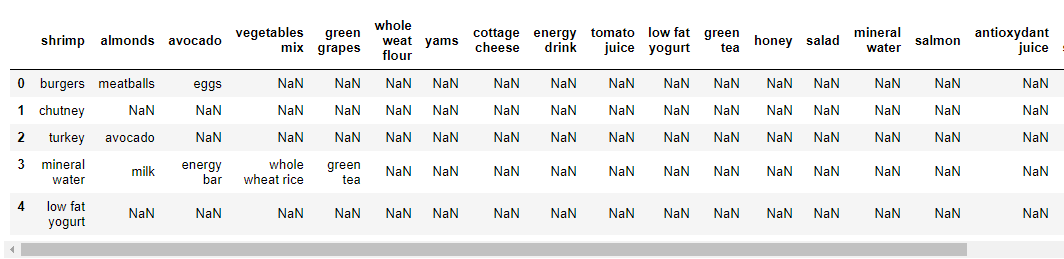
A snippet of the dataset is shown in the above screenshot. If you carefully look at the data, we can see that the header is actually the first transaction. Each row corresponds to a transaction and each column corresponds to an item purchased in that specific transaction. The NaN tells us that the item represented by the column was not purchased in that specific transaction.

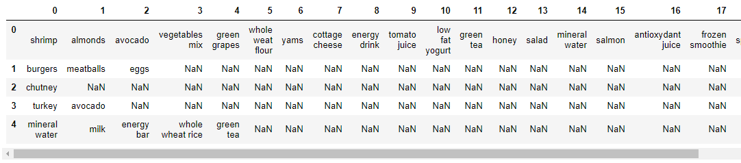
In this dataset there is no header row. But by default, pd.read_csv function treats first row as header. To get rid of this problem, add header=None option to pd.read_csv function, as shown below:

store_data = pd.read_csv('D:\\Datasets\\store_data.csv', header=None)

Now execute the head() function:

store_data.head()

In this updated output you will see that the first line is now treated as a record instead of header as shown below:

Now we will use the Apriori algorithm to find out which items are commonly sold together, so that store owner can take action to place the related items together or advertise them together in order to have increased profit.

Data Proprocessing

The Apriori library we are going to use requires our dataset to be in the form of a list of lists, where the whole dataset is a big list and each transaction in the dataset is an inner list within the outer big list. Currently we have data in the form of a pandas dataframe. To convert our pandas dataframe into a list of lists, execute the following script:

records = []
for i in range(0, 7501):
    records.append([str(store_data.values[i,j]) for j in range(0, 20)])

Applying Apriori

The next step is to apply the Apriori algorithm on the dataset. To do so, we can use the apriori class that we imported from the apyori library.

The apriori class requires some parameter values to work. The first parameter is the list of list that you want to extract rules from. The second parameter is the min_support parameter. This parameter is used to select the items with support values greater than the value specified by the parameter. Next, the min_confidence parameter filters those rules that have confidence greater than the confidence threshold specified by the parameter. Similarly, the min_lift parameter specifies the minimum lift value for the short listed rules. Finally, the min_length parameter specifies the minimum number of items that you want in your rules.

Let's suppose that we want rules for only those items that are purchased at least 5 times a day, or 7 x 5 = 35 times in one week, since our dataset is for a one-week time period. The support for those items can be calculated as 35/7500 = 0.0045. The minimum confidence for the rules is 20% or 0.2. Similarly, we specify the value for lift as 3 and finally min_length is 2 since we want at least two products in our rules. These values are mostly just arbitrarily chosen, so you can play with these values and see what difference it makes in the rules you get back out.

Execute the following script:

association_rules = apriori(records, min_support=0.0045, min_confidence=0.2, min_lift=3, min_length=2)
association_results = list(association_rules)

In the second line here we convert the rules found by the apriori class into a list since it is easier to view the results in this form.

Viewing the Results

Let's first find the total number of rules mined by the apriori class. Execute the following script:

print(len(association_rules))

The script above should return 48. Each item corresponds to one rule.

Let's print the first item in the association_rules list to see the first rule. Execute the following script:

print(association_rules[0])

The output should look like this:

RelationRecord(items=frozenset({'light cream', 'chicken'}), support=0.004532728969470737, ordered_statistics[OrderedStatistic(items_base=frozenset({'light cream'}), items_add=frozenset({'chicken'}), confidence=0.29059829059829057, lift=4.84395061728395)])

The first item in the list is a list itself containing three items. The first item of the list shows the grocery items in the rule.

For instance from the first item, we can see that light cream and chicken are commonly bought together. This makes sense since people who purchase light cream are careful about what they eat hence they are more likely to buy chicken i.e. white meat instead of red meat i.e. beef. Or this could mean that light cream is commonly used in recipes for chicken.

The support value for the first rule is 0.0045. This number is calculated by dividing the number of transactions containing light cream divided by total number of transactions. The confidence level for the rule is 0.2905 which shows that out of all the transactions that contain light cream, 29.05% of the transactions also contain chicken. Finally, the lift of 4.84 tells us that chicken is 4.84 times more likely to be bought by the customers who buy light cream compared to the default likelihood of the sale of chicken.

The following script displays the rule, the support, the confidence, and lift for each rule in a more clear way:

for item in association_rules:

    # first index of the inner list
    # Contains base item and add item
    pair = item[0] 
    items = [x for x in pair]
    print("Rule: " + items[0] + " -> " + items[1])

    #second index of the inner list
    print("Support: " + str(item[1]))

    #third index of the list located at 0th
    #of the third index of the inner list

    print("Confidence: " + str(item[2][0][2]))
    print("Lift: " + str(item[2][0][3]))
    print("=====================================")

If you execute the above script, you will see all the rules returned by the apriori class. The first four rules returned by the apriori class look like this:

Rule: light cream -> chicken
Support: 0.004532728969470737
Confidence: 0.29059829059829057
Lift: 4.84395061728395
=====================================
Rule: mushroom cream sauce -> escalope
Support: 0.005732568990801126
Confidence: 0.3006993006993007
Lift: 3.790832696715049
=====================================
Rule: escalope -> pasta
Support: 0.005865884548726837
Confidence: 0.3728813559322034
Lift: 4.700811850163794
=====================================
Rule: ground beef -> herb & pepper
Support: 0.015997866951073192
Confidence: 0.3234501347708895
Lift: 3.2919938411349285
=====================================

We have already discussed the first rule. Let's now discuss the second rule. The second rule states that mushroom cream sauce and escalope are bought frequently. The support for mushroom cream sauce is 0.0057. The confidence for this rule is 0.3006 which means that out of all the transactions containing mushroom, 30.06% of the transactions are likely to contain escalope as well. Finally, lift of 3.79 shows that the escalope is 3.79 more likely to be bought by the customers that buy mushroom cream sauce, compared to its default sale.

Conclusion

Association rule mining algorithms such as Apriori are very useful for finding simple associations between our data items. They are easy to implement and have high explain-ability. However for more advanced insights, such those used by Google or Amazon etc., more complex algorithms, such as recommender systems, are used. However, you can probably see that this method is a very simple way to get basic associations if that's all your use-case needs.