
Introduction
This article is an introduction to the Pearson Correlation Coefficient, its manual calculation and its computation via Python's numpy module.
The Pearson correlation coefficient measures the linear association between variables. Its value can be interpreted like so:
- +1 - Complete positive correlation
- +0.8 - Strong positive correlation
- +0.6 - Moderate positive correlation
- 0 - no correlation whatsoever
- -0.6 - Moderate negative correlation
- -0.8 - Strong negative correlation
- -1 - Complete negative correlation
We'll illustrate how the correlation coefficient varies with different types of associations. In this article, we'll also show that zero correlation does not always mean zero associations. Non-linearly related variables may have correlation coefficients close to zero.
What is The Pearson Correlation Coefficient?
The Pearson's Correlation Coefficient is also known as the Pearson Product-Moment Correlation Coefficient. It is a measure of the linear relationship between two random variables - X and Y. Mathematically, if (σXY) is the covariance between X and Y, and (σX) is the standard deviation of X, then the Pearson's correlation coefficient ρ is given by:
$$
\rho_{X,Y} = \frac{\sigma_{XY}}{\sigma_X \sigma_Y}
$$
As the covariance is always smaller than the product of the individual standard deviations, the value of ρ varies between -1 and +1. From the above we can also see that the correlation of a variable with itself is one:
$$
\rho_{X,X} = \frac{\sigma_{XX}}{\sigma_X \sigma_X} = 1
$$
Before we start writing code, let's do a short example to see how this coefficient is computed.
How is the Pearson Correlation Coefficient Computed?
Suppose we are given some observations of the random variables X and Y. If you plan to implement everything from scratch or do some manual calculations, then you need the following when given X and Y:
Let's use the above to compute the correlation. We'll use the biased estimate of covariance and standard deviations. This won't affect the value of the correlation coefficient being computed as the number of observations cancels out in the numerator and denominator:
Pearson Correlation Coefficient in Python Using NumPy
The Pearson Correlation coefficient can be computed in Python using the corrcoef() method from NumPy.
The input for this function is typically a matrix, say of size mxn, where:
- Each column represents the values of a random variable
- Each row represents a single sample of
nrandom variables nrepresent the total number of different random variablesmrepresents the total number of samples for each variable
For n random variables, it returns an nxn square matrix M, with M(i,j) indicating the correlation coefficient between the random variable i and j. As the correlation coefficient between a variable and itself is 1, all diagonal entries (i,i) are equal to one.
In short:
Note that the correlation matrix is symmetric as correlation is symmetric, i.e., M(i,j) = M(j,i). Let's take our simple example from the previous section and see how to use corrcoef() with numpy.
First, let's import the numpy module, alongside the pyplot module from Matplotlib. We'll be using Matplotlib to visualize the correlation later on:
import numpy as np
import matplotlib.pyplot as plt
We'll use the same values from the manual example from before. Let's store that into x_simple and compute the correlation matrix:
x_simple = np.array([-2, -1, 0, 1, 2])
y_simple = np.array([4, 1, 3, 2, 0])
my_rho = np.corrcoef(x_simple, y_simple)

print(my_rho)
The following is the output correlation matrix. Note the ones on the diagonals, indicating that the correlation coefficient of a variable with itself is one:
[[ 1.  -0.7]
[-0.7  1. ]]
Positive and Negative Correlation Examples
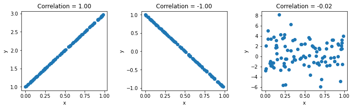
Let's visualize the correlation coefficients for a few relationships. First, we'll have a complete positive (+1) and complete negative (-1) correlation between two variables. Then, we'll generate two random variables, so the correlation coefficient should by all means be close to zero, unless the randomness accidentally has some correlation, which is highly unlikely.
We'll use a seed so that this example is repeatable when calling the RandomState from NumPy:
seed = 13
rand = np.random.RandomState(seed)

x = rand.uniform(0,1,100)
x = np.vstack((x,x*2+1))
x = np.vstack((x,-x[0,]*2+1))
x = np.vstack((x,rand.normal(1,3,100)))
The first rand.uniform() call generates a random uniform distribution:
[7.77702411e-01 2.37541220e-01 8.24278533e-01 9.65749198e-01
 9.72601114e-01 4.53449247e-01 6.09042463e-01 7.75526515e-01
 6.41613345e-01 7.22018230e-01 3.50365241e-02 2.98449471e-01
 5.85124919e-02 8.57060943e-01 3.72854028e-01 6.79847952e-01
 2.56279949e-01 3.47581215e-01 9.41277008e-03 3.58333783e-01
 9.49094182e-01 2.17899009e-01 3.19391366e-01 9.17772386e-01
 3.19036664e-02 6.50845370e-02 6.29828999e-01 8.73813443e-01
 8.71573230e-03 7.46577237e-01 8.12841171e-01 7.57174462e-02
 6.56455335e-01 5.09262200e-01 4.79883391e-01 9.55574145e-01
 1.20335695e-05 2.46978701e-01 7.12232678e-01 3.24582050e-01
 2.76996356e-01 6.95445453e-01 9.18551748e-01 2.44475702e-01
 4.58085817e-01 2.52992683e-01 3.79333291e-01 6.04538829e-01
 7.72378760e-01 6.79174968e-02 6.86085079e-01 5.48260097e-01
 1.37986053e-01 9.87532192e-02 2.45559105e-01 1.51786663e-01
 9.25994479e-01 6.80105016e-01 2.37658922e-01 5.68885253e-01
 5.56632051e-01 7.27372109e-02 8.39708510e-01 4.05319493e-01
 1.44870989e-01 1.90920059e-01 4.90640137e-01 7.12024374e-01
 9.84938458e-01 8.74786502e-01 4.99041684e-01 1.06779994e-01
 9.13212807e-01 3.64915961e-01 2.26587877e-01 8.72431862e-01
 1.36358352e-01 2.36380160e-01 5.95399245e-01 5.63922609e-01
 9.58934732e-01 4.53239333e-01 1.28958075e-01 7.60567677e-01
 2.01634075e-01 1.75729863e-01 4.37118013e-01 3.40260803e-01
 9.67253109e-01 1.43026077e-01 8.44558533e-01 6.69406140e-01
 1.09304908e-01 8.82535400e-02 9.66462041e-01 1.94297485e-01
 8.19000600e-02 2.69384695e-01 6.50130518e-01 5.46777245e-01]
Check out our hands-on, practical guide to learning Git, with best-practices, industry-accepted standards, and included cheat sheet. Stop Googling Git commands and actually learn it!
Then, we can call vstack() to vertically stack other arrays to it. This way, we can stack a bunch of variables like the ones above in the same x reference and access them sequentially.
After the first uniform distribution, we've stacked a few variable sets vertically - the second one has a complete positive relation to the first one, the third one has a complete negative correlation to the first one, and the fourth one is fully random, so it should have a ~0 correlation.
When we have a single x reference like this, we can calculate the correlation for each of the elements in the vertical stack by passing it alone to np.corrcoef():
rho = np.corrcoef(x)

fig, ax = plt.subplots(nrows=1, ncols=3, figsize=(12, 3))
for i in [0,1,2]:
    ax[i].scatter(x[0,],x[1+i,])
    ax[i].title.set_text('Correlation = ' + "{:.2f}".format(rho[0,i+1]))
    ax[i].set(xlabel='x',ylabel='y')
fig.subplots_adjust(wspace=.4)
plt.show()
Understanding Pearson's Correlation Coefficient Changes
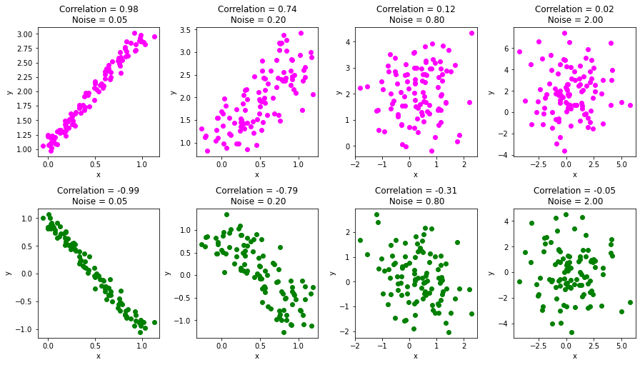
Just to see how the correlation coefficient changes with a change in the relationship between the two variables, let's add some random noise to the x matrix generated in the previous section and re-run the code.
In this example, we'll slowly add varying degrees of noise to the correlation plots, and calculating the correlation coefficients on each step:
fig, ax = plt.subplots(nrows=2, ncols=4, figsize=(15, 8))

for noise, i in zip([0.05,0.2,0.8,2],[0,1,2,3]):
    # Add noise
    x_with_noise = x+rand.normal(0,noise,x.shape)

    # Compute correlation
    rho_noise = np.corrcoef(x_with_noise)

    # Plot column wise. Positive correlation in row 0 and negative in row 1
    ax[0,i].scatter(x_with_noise[0,],x_with_noise[1,],color='magenta')
    ax[1,i].scatter(x_with_noise[0,],x_with_noise[2,],color='green')
    ax[0,i].title.set_text('Correlation = ' + "{:.2f}".format(rho_noise[0,1])
                        + '\n Noise = ' + "{:.2f}".format(noise) )
    ax[1,i].title.set_text('Correlation = ' + "{:.2f}".format(rho_noise[0,2])
                        + '\n Noise = ' + "{:.2f}".format(noise))
    ax[0,i].set(xlabel='x',ylabel='y')
    ax[1,i].set(xlabel='x',ylabel='y')

fig.subplots_adjust(wspace=0.3,hspace=0.4)
plt.show()
A Common Pitfall: Associations with No Correlation
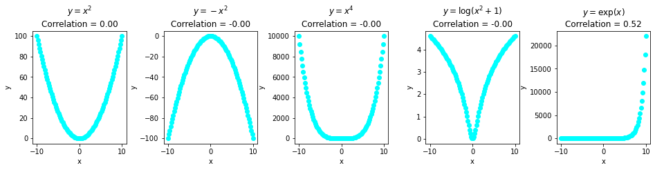
There is a common misconception that zero correlation implies no association. Let's clarify that correlation strictly measures the linear relationship between two variables.
The examples below show variables which are non-linearly associated with each other but have zero correlation.
The last example of (y=ex) has a correlation coefficient of around 0.52, which is again not a reflection of the true association between the two variables:
# Create a data matrix
x_nonlinear = np.linspace(-10,10,100)
x_nonlinear = np.vstack((x_nonlinear,x_nonlinear*x_nonlinear))
x_nonlinear = np.vstack((x_nonlinear,-x_nonlinear[0,]**2))
x_nonlinear = np.vstack((x_nonlinear,x_nonlinear[0,]**4))
x_nonlinear = np.vstack((x_nonlinear,np.log(x_nonlinear[0,]**2+1)))
x_nonlinear = np.vstack((x_nonlinear,np.exp(x_nonlinear[0,])))

# Compute the correlation
rho_nonlinear = np.corrcoef(x_nonlinear)

# Plot the data
fig, ax = plt.subplots(nrows=1, ncols=5, figsize=(16, 3))
title = ['$y=x^2$','$y=-x^2$','$y=x^4$','$y=\log(x^2+1)$','$y=\exp(x)$']
for i in [0,1,2,3,4]:
    ax[i].scatter(x_nonlinear[0,],x_nonlinear[1+i,],color='cyan')
    ax[i].title.set_text(title[i] + '\n' +
                         'Correlation = ' + "{:.2f}".format(rho_nonlinear[0,i+1]))
    ax[i].set(xlabel='x',ylabel='y')
fig.subplots_adjust(wspace=.4)
plt.show()
Conclusions
In this article, we discussed the Pearson correlation coefficient. We used the corrcoef() method from Python's numpy module to compute its value.
If random variables have high linear associations then their correlation coefficient is close to +1 or -1. On the other hand, statistically independent variables have correlation coefficients close to zero.
We also demonstrated that non-linear associations can have a correlation coefficient zero or close to zero, implying that variables having high associations may not have a high value of the Pearson correlation coefficient.

