Dijkstra's Algorithm


Dijkstra's algorithm is an designed to find the shortest paths between nodes in a graph. It was designed by a Dutch computer scientist, Edsger Wybe Dijkstra, in 1956, when pondering the shortest route from Rotterdam to Groningen. It was published three years later.
Note: Dijkstra's algorithm has seen changes throughout the years and various versions and variations exist. Originally - it was used to calculate the shortest path between two nodes. Due to the way it works - it was adapted to calculate the shortest path between a starting node and every other node in the graph. This way - it can be used to produce a shortest-path tree that consists of the shortest path between two nodes, as well as all other nodes. You can then prune away the trees you're not interested in, getting the shortest path between two nodes, but you'll inevitably have to calculate the entire tree, which is a drawback of Dijkstra's algorithm that makes it unfit for large graphs.
We'll be focusing on the latter implementation in the lesson.
In this lesson, we'll take a look at Dijkstra's algorithm, the intuition behind it and then implement it in Python.
Dijkstra's Algorithm - Theory and Intuition
Dijkstra's algorithm works on undirected, connected, weighted graphs.
In the beginning, we'll want to create a set of visited vertices, to keep track of all of the vertices that have been assigned their correct shortest path. We will also need to set "costs" of all vertices in the graph (lengths of the current shortest path that leads to it).
All of the costs will be set to 'infinity' at the beginning, to make sure that every other cost we may compare it to would be smaller than the starting one. The only exception is the cost of the first, starting vertex - this vertex will have a cost of 0, because it has no path to itself - marked as node s.
Then, we repeat two main steps until the graph is traversed (as long as there are vertices without the shortest path assigned to them):
- We pick a vertex with the shortest current cost, visit it, and add it to the visited vertices set.
- We update the costs of all its adjacent vertices that are not visited yet. For every edge between
nandmwheremis unvisited - if thecheapestPath(s, n)+cheapestPath(n,m)<cheapestPath(s,m), update the cheapest path betweensandmto equalcheapestPath(s,n)+cheapestPath(n,m).
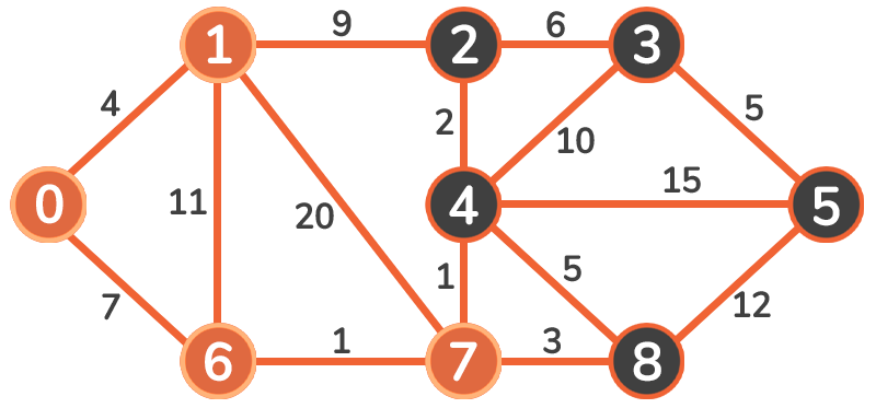
Since this might be a bit difficult to wrap one's head around - let's visualize the process before implementing it! Here's an undirected, weighted, connected graph:

Let's say that Vertex 0 is our starting point. We are going to set the initial costs of vertices in this graph to infinity, except for the starting vertex:
| vertex | cost to get to it from vertex 0 |
|---|---|
| 0 | 0 |
| 1 | inf |
| 2 | inf |
| 3 | inf |
| 4 | inf |
| 5 | inf |
| 6 | inf |
| 7 | inf |
| 8 | inf |
We pick the vertex with a minimum cost - that is Vertex 0. We will mark it as visited and add it to our set of visited vertices. The starting node will always have the lowest cost so it will always be the first one to be added:

Then, we will update the cost of adjacent vertices (1 and 6). Since 0 + 4 < infinity and 0 + 7 < infinity, we update the costs to these vertices:
| vertex | cost to get to it from vertex 0 |
|---|---|
| 0 | 0 |
| 1 | 4 |
| 2 | inf |
| 3 | inf |
| 4 | inf |
| 5 | inf |
| 6 | 7 |
| 7 | inf |
| 8 | inf |
Now we visit the next smallest cost vertex. The weight of 4 is lower than 7 so we traverse to Vertex 1:

Upon traversing, we mark it as visited, and then observe and update the adjacent vertices: 2, 6, and 7:
- Since
4 + 9 < infinity, new cost of vertex 2 will be 13 - Since
4 + 11 > 7, the cost of vertex 6 will remain 7 - Since
4 + 20 < infinity, new cost of vertex 7 will be 24
These are our new costs:
| vertex | cost to get to it from vertex 0 |
|---|---|
| 0 | 0 |
| 1 | 4 |
| 2 | 13 |
| 3 | inf |
| 4 | inf |
| 5 | inf |
| 6 | 7 |
| 7 | 24 |
| 8 | inf |
The next vertex we're going to visit is Vertex 6. We mark it as visited and update its adjacent vertices' costs:

| vertex | cost to get to it from vertex 0 |
|---|---|
| 0 | 0 |
| 1 | 4 |
| 2 | 13 |
| 3 | inf |
| 4 | inf |
| 5 | inf |
| 6 | 7 |
| 7 | 8 |
| 8 | inf |
The process is continued to Vertex 7:
| vertex | cost to get to it from vertex 0 |
|---|---|
| 0 | 0 |
| 1 | 4 |
| 2 | 13 |
| 3 | inf |
| 4 | 9 |
| 5 | inf |
| 6 | 7 |
| 7 | 8 |
| 8 | 11 |
And again, to Vertex 4:

| vertex | cost to get to it from vertex 0 |
|---|---|
| 0 | 0 |
| 1 | 4 |
| 2 | 11 |
| 3 | 19 |
| 4 | 9 |
| 5 | 24 |
| 6 | 7 |
| 7 | 8 |
| 8 | 11 |
And again, to Vertex 2:

The only vertex we're going to consider is Vertex 3. Since 11 + 6 < 19, the cost of vertex 3 is updated.
Then, we proceed to Vertex 8:

Finally, we're updating the Vertex 5:
| vertex | cost to get to it from vertex 0 |
|---|---|
| 0 | 0 |
| 1 | 4 |
| 2 | 11 |
| 3 | 17 |
| 4 | 9 |
| 5 | 24 |
| 6 | 7 |
| 7 | 8 |
| 8 | 11 |
We've updated the vertices in the loop-like structure in the end - so now we just have to traverse it - first to Vertex 3:

And finally, to the Vertex 5:

There are no more unvisited vertices that may need an update. Our final costs represents the shortest paths from node 0 to every other node in the graph:
| vertex | cost to get to it from vertex 0 |
|---|---|
| 0 | 0 |
| 1 | 4 |
| 2 | 11 |
| 3 | 17 |
| 4 | 9 |
| 5 | 24 |
| 6 | 7 |
| 7 | 8 |
| 8 | 11 |
Implement Dijkstra's Algorithm in Python
Now that we've gone over the step-by-step process, let's see how we can implement Dijkstra's algorithm in Python! To sort and keep track of the vertices we haven't visited yet - we'll use a PriorityQueue:
from queue import PriorityQueue
Now, we'll implement a constructor for a class called Graph:
class Graph:
    def __init__(self, num_of_vertices):
        self.v = num_of_vertices
        self.edges = [[-1 for i in range(num_of_vertices)] for j in range(num_of_vertices)]
        self.visited = []
In this simple parametrized constructor, we provided the number of vertices in the graph as an argument, and we initialized three fields:
v: Represents the number of vertices in the graph.edges: Represents the list of edges in the form of a matrix. For nodesuandv,self.edges[u][v] = weightof the edge.visited: A set which will contain the visited vertices.
Now, let's define a function which is going to add an edge to a graph:
    def add_edge(self, u, v, weight):
        self.edges[u][v] = weight
        self.edges[v][u] = weight
With our graph definition out of the way - let's define Dijkstra's algorithm:
def dijkstra(graph, start_vertex):
    D = {v:float('inf') for v in range(graph.v)}
    D[start_vertex] = 0

    pq = PriorityQueue()
    pq.put((0, start_vertex))

    while not pq.empty():
        (dist, current_vertex) = pq.get()
        graph.visited.append(current_vertex)

        for neighbor in range(graph.v):
            if graph.edges[current_vertex][neighbor] != -1:
                distance = graph.edges[current_vertex][neighbor]
                if neighbor not in graph.visited:
                    old_cost = D[neighbor]
                    new_cost = D[current_vertex] + distance
                    if new_cost < old_cost:
                        pq.put((new_cost, neighbor))
                        D[neighbor] = new_cost
    return D
In this code, we first created a list D of the size v. The entire list is initialized to infinity. This is going to be a list where we keep the shortest paths from start_vertex to all of the other nodes.
We set the value of the start vertex to 0, since that is its distance from itself. Then, we initialize a priority queue, which we will use to quickly sort the vertices from the least to most distant. We put the start vertex in the priority queue. Now, for each vertex in the priority queue, we will first mark them as visited, and then we will iterate through their neighbors.
If the neighbor is not visited, we will compare its old cost and its new cost. The old cost is the current value of the shortest path from the start vertex to the neighbor, while the new cost is the value of the sum of the shortest path from the start vertex to the current vertex and the distance between the current vertex and the neighbor. If the new cost is lower than the old cost, we put the neighbor and its cost to the priority queue, and update the list where we keep the shortest paths accordingly.
Finally, after all of the vertices are visited and the priority queue is empty, we return the list D.
Let's initialize a graph we've used before to validate our manual steps, and test the algorithm:
g = Graph(9)
g.add_edge(0, 1, 4)
g.add_edge(0, 6, 7)
g.add_edge(1, 6, 11)
g.add_edge(1, 7, 20)
g.add_edge(1, 2, 9)
g.add_edge(2, 3, 6)
g.add_edge(2, 4, 2)
g.add_edge(3, 4, 10)
g.add_edge(3, 5, 5)
g.add_edge(4, 5, 15)
g.add_edge(4, 7, 1)
g.add_edge(4, 8, 5)
g.add_edge(5, 8, 12)
g.add_edge(6, 7, 1)
g.add_edge(7, 8, 3)
Now, we will simply call the function that performs Dijkstra's algorithm on this graph and print out the results:
D = dijkstra(g, 0)

print(D)
# {0: 0, 1: 4, 2: 11, 3: 17, 4: 9, 5: 22, 6: 7, 7: 8, 8: 11}
Or, we could format it a bit more nicely:
for vertex in range(len(D)):
    print("Distance from vertex 0 to vertex", vertex, "is", D[vertex])
Once we compile the program, we will get this output:
Distance from vertex 0 to vertex 0 is 0
Distance from vertex 0 to vertex 1 is 4
Distance from vertex 0 to vertex 2 is 11
Distance from vertex 0 to vertex 3 is 17
Distance from vertex 0 to vertex 4 is 9
Distance from vertex 0 to vertex 5 is 22
Distance from vertex 0 to vertex 6 is 7
Distance from vertex 0 to vertex 7 is 8
Distance from vertex 0 to vertex 8 is 11
The distance between the starting node and each other node in the tree is calculated and output.
Time Complexity
In this algorithm, we pass each edge once, which results in time complexity of O(|E|), where |E| represents the number of edges.
We also visit each node once, which results in time complexity of O(|V|), where |V| represents the number of vertices. Each vertex will be put in a priority queue, where finding the next closest vertex is going to be done in constant O(1) time. However, we use O(Vlog|V|) time to sort the vertices in this priority queue.
This results in time complexity of this algorithm being O(|E|+|V|log|V|).