Dynamic Programming in Java

Introduction

Dynamic Programming is typically used to optimize recursive algorithms, as they tend to scale exponentially. The main idea is to break down complex problems (with many recursive calls) into smaller subproblems and then save them into memory so that we don't have to recalculate them each time we use them.

What is Dynamic Programming?

Dynamic programming is a programming principle where a very complex problem can be solved by dividing it into smaller subproblems. This principle is very similar to recursion, but with a key difference, every distinct subproblem has to be solved only once.

To understand what this means, we first have to understand the problem of solving recurrence relations. Every single complex problem can be divided into very similar subproblems, this means we can construct a recurrence relation between them.

Let's take a look at an example we all are familiar with, the Fibonacci sequence! The Fibonacci sequence is defined with the following recurrence relation:

$$
fibonacci(n)=fibonacci(n-1)+fibonacci(n-2)
$$

Note: A recurrence relation is an equation that recursively defines a sequence where the next term is a function of the previous terms. The Fibonacci sequence is a great example of this.

So, if we want to find the n-th number in the Fibonacci sequence, we have to know the two numbers preceding the n-th in the sequence.

However, every single time we want to calculate a different element of the Fibonacci sequence, we have have certain duplicate calls in our recursive calls, as can be seen in following image, where we calculate Fibonacci(5):

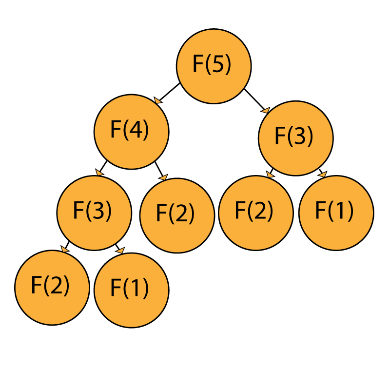
For example, if we want to calculate F(5), we obviously need to calculate F(4) and F(3) as a prerequisite. However, to calculate F(4), we need to calculate F(3) and F(2), which in turn requires us to calculate F(2) and F(1) in order to get F(3) – and so on.

This leads to many repeated calculations, which are essentially redundant and slow down the algorithm significantly. To solve this issue, we're introducing ourselves to Dynamic Programming.

In this approach, we model a solution as if we were to solve it recursively, but we solve it from the ground up, memoizing the solutions to the subproblems (steps) we take to reach the top.

Therefore, for the Fibonacci sequence, we first solve and memoize F(1) and F(2), then calculate F(3) using the two memoized steps, and so on. This means that the calculation of every individual element of the sequence is O(1), because we already know the former two.

When solving a problem using dynamic programming, we have to follow three steps:

• Determine the recurrence relation that applies to said problem
• Initialize the memory/array/matrix's starting values
• Make sure that when we make a "recursive call" (access the memoized solution of a subproblem) it's always solved in advance

Following these rules, let's take a look at some examples of algorithms that use dynamic programming.

Rod Cutting Algorithm

Let's start with something simple:

Given a rod of length n and an array that contains prices of all pieces of size smaller than n. Determine the maximum value obtainable by cutting up the rod and selling the pieces.

Naive Solution

This problem is practically tailor-made for dynamic programming, but because this is our first real example, let's see how many fires we can start by letting this code run:

public class naiveSolution {
    static int getValue(int[] values, int length) {
        if (length <= 0)
            return 0;
        int tmpMax = -1;
        for (int i = 0; i < length; i++) {
            tmpMax = Math.max(tmpMax, values[i] + getValue(values, length - i - 1));
        }
        return tmpMax;
    }

    public static void main(String[] args) {
        int[] values = new int[]{3, 7, 1, 3, 9};
        int rodLength = values.length;

        System.out.println("Max rod value: " + getValue(values, rodLength));
    }
}

Output:

Max rod value: 17

This solution, while correct, is highly inefficient. Recursive calls aren't memoized so the poor code has to solve the same subproblem every time there's a single overlapping solution.

Dynamic Approach

Utilizing the same basic principle from above, but adding memoization and excluding recursive calls, we get the following implementation:

public class dpSolution {
    static int getValue(int[] values, int rodLength) {
        int[] subSolutions = new int[rodLength + 1];

        for (int i = 1; i <= rodLength; i++) {
            int tmpMax = -1;
            for (int j = 0; j < i; j++)
                tmpMax = Math.max(tmpMax, values[j] + subSolutions[i - j - 1]);
            subSolutions[i] = tmpMax;
        }
        return subSolutions[rodLength];
    }

    public static void main(String[] args) {
        int[] values = new int[]{3, 7, 1, 3, 9};
        int rodLength = values.length;

        System.out.println("Max rod value: " + getValue(values, rodLength));
    }
}

Output:

Max rod value: 17

As we can see, the resulting outputs are the same, only with different time/space complexity.

We eliminate the need for recursive calls by solving the subproblems from the ground-up, utilizing the fact that all previous subproblems to a given problem are already solved.

Performance Boost

Just to give a perspective of how much more efficient the Dynamic approach is, let's try running the algorithm with 30 values.

The Naive solution took ~5.2s to execute whereas the Dynamic solution took ~0.000095s to execute.

Simplified Knapsack Problem

The Simplified Knapsack problem is a problem of optimization, for which there is no one solution. The question for this problem would be - "Does a solution even exist?":

Given a set of items, each with a weight w1, w2... determine the number of each item to put in a knapsack so that the total weight is less than or equal to a given limit K.

So let's take a step back and figure out how we will represent the solutions to this problem. First, let's store the weights of all the items in an array W.

Next, let's say that there are n items and we'll enumerate them with numbers from 1 to n, so the weight of the i-th item is W[i].

We'll form a matrix M of (n+1)x(K+1) dimensions. M[x][y] corresponds to the solution of the knapsack problem, but only including the first x items of the beginning array, and with a maximum capacity of y.

Example

Let's say we have 3 items, with the weights being w1=2kg, w2=3kg, and w3=4kg.

Utilizing the method above, we can say that M[1][2] is a valid solution. This means that we are trying to fill a knapsack with a capacity of 2kg with just the first item from the weight array (w1).

While in M[3][5] we are trying to fill up a knapsack with a capacity of 5kg using the first 3 items of the weight array (w1,w2,w3). This isn't a valid solution, since we're overfitting it.

Matrix Initialization

There are 2 things to note when filling up the matrix:

Does a solution exist for the given subproblem (M[x][y].exists) AND does the given solution include the latest item added to the array (M[x][y].includes).

Therefore, initialization of the matrix is quite easy, M[0][k].exists is always false, if k > 0, because we didn't put any items in a knapsack with k capacity.

On the other hand, M[0][0].exists = true, because the knapsack should be empty to begin with since k = 0, and therefore we can't put anything in and this is a valid solution.

Furthermore, we can say that M[k][0].exists = true but also M[k][0].includes = false for every k.

Note: Just because a solution exists for a given M[x][y], it doesn't necessarily mean that that particular combination is the solution. In the case of M[10][0], a solution exists - not including any of the 10 elements. This is why M[10][0].exists = true but M[10][0].includes = false.

Algorithm Principle

Next, let's construct the recurrence relation for M[i][k] with the following pseudo-code:

if (M[i-1][k].exists == True):
    M[i][k].exists = True
    M[i][k].includes = False
elif (k-W[i]>=0):
    if(M[i-1][k-W[i]].exists == true):
        M[i][k].exists = True
        M[i][k].includes = True
else:
    M[i][k].exists = False

So the gist of the solution is dividing the subproblem into two cases:

1. When a solution exists for the first i-1 elements, for capacity k
2. When a solution exists for the first i-1 elements, but for capacity k-W[i]

The first case is self-explanatory, we already have a solution to the problem.

The second case refers to knowing the solution for the first i-1 elements, but the capacity is with exactly one i-th element short of being full, which means we can just add one i-th element, and we have a new solution!

Implementation

In this implementation, to make things easier, we'll make the class Element for storing elements:

public class Element {
    private boolean exists;
    private boolean includes;

    public Element(boolean exists, boolean includes) {
        this.exists = exists;
        this.includes = includes;
    }

    public Element(boolean exists) {
        this.exists = exists;
        this.includes = false;
    }

    public boolean isExists() {
        return exists;
    }

    public void setExists(boolean exists) {
        this.exists = exists;
    }

    public boolean isIncludes() {
        return includes;
    }

    public void setIncludes(boolean includes) {
        this.includes = includes;
    }
}

Now we can dive into the main class:

public class Knapsack {
    public static void main(String[] args) {
        Scanner scanner = new Scanner (System.in);

        System.out.println("Insert knapsack capacity:");
        int k = scanner.nextInt();

        System.out.println("Insert number of items:");
        int n = scanner.nextInt();

        System.out.println("Insert weights: ");
        int[] weights = new int[n + 1];

        for (int i = 1; i <= n; i++) {
            weights[i] = scanner.nextInt();
        }

        Element[][] elementMatrix = new Element[n + 1][k + 1];

        elementMatrix[0][0] = new Element(true);

        for (int i = 1; i <= k; i++) {
            elementMatrix[0][i] = new Element(false);
        }

        for (int i = 1; i <= n; i++) {
            for (int j = 0; j <= k; j++) {
                elementMatrix[i][j] = new Element(false);
                if (elementMatrix[i - 1][j].isExists()) {
                    elementMatrix[i][j].setExists(true);
                    elementMatrix[i][j].setIncludes(false);
                } else if (j >= weights[i]) {
                    if (elementMatrix[i - 1][j - weights[i]].isExists()) {
                        elementMatrix[i][j].setExists(true);
                        elementMatrix[i][j].setIncludes(true);
                    }
                }
            }
        }

        System.out.println(elementMatrix[n][k].isExists());
    }
}

The only thing that's left is reconstruction of the solution, in the class above, we know that a solution EXISTS. However, we don't know what it is.

For reconstruction we use the following code:

List<Integer> solution = new ArrayList<>(n);

if (elementMatrix[n][k].isExists()) {
    int i = n;
    int j = k;
    while (j > 0 && i > 0) {
        if (elementMatrix[i][j].isIncludes()) {
            solution.add(i);
            j = j - weights[i];
        }
        i = i - 1;
    }
}

System.out.println("The elements with the following indexes are in the solution:\n" + (solution.toString()));

Output:

Insert knapsack capacity:
12
Insert number of items:
5
Insert weights:
9 7 4 10 3
true
The elements with the following indexes are in the solution:
[5, 1]

A simple variation of the knapsack problem is filling a knapsack without value optimization, but now with unlimited amounts of every individual item.

This variation can be solved by making a simple adjustment to our existing code:

// Old code for simplified knapsack problem
else if (j >= weights[i]) {
    if (elementMatrix[i - 1][j - weights[i]].isExists()) {
        elementMatrix[i][j].setExists(true);
        elementMatrix[i][j].setIncludes(true);
    }
}

// New code, note that we're searching for a solution in the same
// row (i-th row), which means we're looking for a solution that
// already has some number of i-th elements (including 0) in it's solution
else if (j >= weights[i]) {
    if (elementMatrix[i][j - weights[i]].isExists()) {
        elementMatrix[i][j].setExists(true);
        elementMatrix[i][j].setIncludes(true);
    }
}

The Traditional Knapsack Problem

Utilizing both previous variations, let's now take a look at the traditional knapsack problem and see how it differs from the simplified variation:

Given a set of items, each with a weight w1, w2... and a value v1, v2... determine the number of each item to include in a collection so that the total weight is less than or equal to a given limit k and the total value is as large as possible.

In the simplified version, every single solution was equally as good. However, now we have a criteria for finding an optimal solution (aka the largest value possible). Keep in mind, this time we have an infinite number of each item, so items can occur multiple times in a solution.

In the implementation we'll be using the old class Element, with an added private field value for storing the largest possible value for a given subproblem:

public class Element {
    private boolean exists;
    private boolean includes;
    private int value;
    // appropriate constructors, getters and setters
}

The implementation is very similar, with the only difference being that now we have to choose the optimal solution judging by the resulting value:

public static void main(String[] args) {
    // Same code as before with the addition of the values[] array
    System.out.println("Insert values: ");
    int[] values = new int[n + 1];

    for (int i=1; i <= n; i++) {
        values[i] = scanner.nextInt();
    }

    Element[][] elementMatrix = new Element[n + 1][k + 1];

    // A matrix that indicates how many newest objects are used
    // in the optimal solution.
    // Example: contains[5][10] indicates how many objects with
    // the weight of W[5] are contained in the optimal solution
    // for a knapsack of capacity K=10
    int[][] contains = new int[n + 1][k + 1];

    elementMatrix[0][0] = new Element(0);

    for (int i = 1; i <= n; i++) {
        elementMatrix[i][0] = new Element(0);
        contains[i][0] = 0;
    }

    for (int i = 1; i <= k; i++) {
        elementMatrix[0][i] = new Element(0);
        contains[0][i] = 0;
    }

    for (int i = 1; i <= n; i++) {
        for (int j = 0; j <= k; j++) {
            elementMatrix[i][j] = new Element(elementMatrix[i - 1][j].getValue());
            contains[i][j] = 0;

            elementMatrix[i][j].setIncludes(false);
            elementMatrix[i][j].setValue(M[i - 1][j].getValue());

            if (j >= weights[i]) {
                if ((elementMatrix[i][j - weights[i]].getValue() > 0 || j == weights[i])) {
                    if (elementMatrix[i][j - weights[i]].getValue() + values[i] > M[i][j].getValue()) {
                        elementMatrix[i][j].setIncludes(true);
                        elementMatrix[i][j].setValue(M[i][j - weights[i]].getValue() + values[i]);
                        contains[i][j] = contains[i][j - weights[i]] + 1;
                    }
                }
            }

            System.out.print(elementMatrix[i][j].getValue() + "/" + contains[i][j] + "  ");
        }

        System.out.println();
    }

    System.out.println("Value: " + elementMatrix[n][k].getValue());
}

Output:

Insert knapsack capacity:
12
Insert number of items:
5
Insert weights:
9 7 4 10 3
Insert values:
1 2 3 4 5
0/0  0/0  0/0  0/0  0/0  0/0  0/0  0/0  0/0  1/1  0/0  0/0  0/0
0/0  0/0  0/0  0/0  0/0  0/0  0/0  2/1  0/0  1/0  0/0  0/0  0/0
0/0  0/0  0/0  0/0  3/1  0/0  0/0  2/0  6/2  1/0  0/0  5/1  9/3
0/0  0/0  0/0  0/0  3/0  0/0  0/0  2/0  6/0  1/0  4/1  5/0  9/0
0/0  0/0  0/0  5/1  3/0  0/0  10/2  8/1  6/0  15/3  13/2  11/1  20/4
Value: 20

Levenshtein Distance

Another very good example of using dynamic programming is Edit Distance or the Levenshtein Distance.

The Levenshtein distance for 2 strings A and B is the number of atomic operations we need to use to transform A into B which are:

1. Character deletion
2. Character insertion
3. Character substitution (technically it's more than one operation, but for the sake of simplicity let's call it an atomic operation)

This problem is handled by methodically solving the problem for substrings of the beginning strings, gradually increasing the size of the substrings until they're equal to the beginning strings.

The recurrence relation we use for this problem is as follows:

c(a,b) being 0 if a==b, and 1 if a!=b.

If you're interested in reading more about Levenshtein Distance, we've already got it covered in Python in another article: Levenshtein Distance and Text Similarity in Python

Implementation

public class editDistance {
    public static void main(String[] args) {
        String s1, s2;
        Scanner scanner = new Scanner(System.in);
        System.out.println("Insert first string:");
        s1 = scanner.next();
        System.out.println("Insert second string:");
        s2 = scanner.next();

        int n, m;
        n = s1.length();
        m = s2.length();

        // Matrix of substring edit distances
        // example: distance[a][b] is the edit distance
        // of the first a letters of s1 and b letters of s2
        int[][] distance = new int[n + 1][m + 1];

        // Matrix initialization:
        // If we want to turn any string into an empty string
        // the fastest way no doubt is to just delete
        // every letter individually.
        // The same principle applies if we have to turn an empty string
        // into a non empty string, we just add appropriate letters
        // until the strings are equal.
        for (int i = 0; i <= n; i++) {
            distance[i][0] = i;
        }
        for (int j = 0; j <= n; j++) {
            distance[0][j] = j;
        }

        // Variables for storing potential values of current edit distance
        int e1, e2, e3, min;

        for (int i = 1; i <= n; i++) {
            for (int j = 1; j <= m; j++) {
                e1 = distance[i - 1][j] + 1;
                e2 = distance[i][j - 1] + 1;
                if (s1.charAt(i - 1) == s2.charAt(j - 1)) {
                    e3 = distance[i - 1][j - 1];
                } else {
                    e3 = distance[i - 1][j - 1] + 1;
                }
                min = Math.min(e1, e2);
                min = Math.min(min, e3);
                distance[i][j] = min;
            }

        }

        System.out.println("Edit distance of s1 and s2 is: " + distance[n][m]);
    }
}

Output:

Insert first string:
man
Insert second string:
machine
Edit distance of s1 and s2 is: 3

Longest Common Subsequence (LCS)

The problem goes as follows:

Given two sequences, find the length of the longest subsequence present in both of them. A subsequence is a sequence that appears in the same relative order, but not necessarily contiguous.

Clarification

If we have two strings, s1 = "MICE" and s2 = "MINCE", the longest common substring would be "MI" or "CE", however, the longest common subsequence would be "MICE" because the elements of the resulting subsequence don't have to be in consecutive order.

Recurrence Relation and General Logic

As we can see, there is only a slight difference between Levenshtein distance and LCS, specifically, in the cost of moves.

In LCS, we have no cost for character insertion and character deletion, which means that we only count the cost for character substitution (diagonal moves), which have a cost of 1 if the two current string characters a[i] and b[j] are the same.

The final cost of LCS is the length of the longest subsequence for the 2 strings, which is exactly what we needed.

Using this logic, we can boil down a lot of string comparison algorithms to simple recurrence relations which utilize the base formula of the Levenshtein distance.

Implementation

public class LCS {
    public static void main(String[] args) {
        String s1 = new String("Hillfinger");
        String s2 = new String("Hilfiger");
        int n = s1.length();
        int m = s2.length();
        int[][] solutionMatrix = new int[n+1][m+1];
        for (int i = 0; i < n; i++) {
            solutionMatrix[i][0] = 0;
        }
        for (int i = 0; i < m; i++) {
            solutionMatrix[0][i] = 0;
        }

        for (int i = 1; i <= n; i++) {
            for (int j = 1; j <= m; j++) {
                int max1, max2, max3;
                max1 = solutionMatrix[i - 1][j];
                max2 = solutionMatrix[i][j - 1];
                if (s1.charAt(i - 1) == s2.charAt(j - 1)) {
                    max3 = solutionMatrix[i - 1][j - 1] + 1;
                } else {
                    max3 = solutionMatrix[i - 1][j - 1];
                }
                int tmp = Math.max(max1, max2);
                solutionMatrix[i][j] = Math.max(tmp, max3);
            }
        }
        
        System.out.println("Length of the longest continuous subsequence: " + solutionMatrix[n][m]);
    }
}

Output:

Length of longest continuous subsequence: 8

Other Problems that Utilize Dynamic Programming

There are a lot more problems that can be solved with dynamic programming, these are just a few of them:

• Partition Problem (coming soon)
• Given a set of integers, find out if it can be divided into two subsets with equal sums
• Subset Sum Problem (coming soon)
• Given a set of positive integers, and a value sum, determine if there is a subset of the given set with sum equal to given sum.
• Coin Change Problem (Total number of ways to get the denomination of coins, coming soon)
• Given an unlimited supply of coins of given denominations, find the total number of distinct ways to get a desired change.
• Total possible solutions to linear equation of k variables (coming soon)
• Given a linear equation of k variables, count the total number of possible solutions of it.
• Find Probability that a Drunkard doesn't fall off a cliff (Kids, do not try this at home)
• Given a linear space representing the distance from a cliff, and providing you know the starting distance of the drunkard from the cliff, and his tendency to go towards the cliff p and away from the cliff 1-p, calculate the probability of his survival.
• Many more...

Conclusion

Dynamic programming is a tool that can save us a lot of computational time in exchange for a bigger space complexity, granted some of them only go halfway (a matrix is needed for memoization, but an ever-changing array is used).

This highly depends on the type of system you're working on, if CPU time is precious, you opt for a memory-consuming solution, on the other hand, if your memory is limited, you opt for a more time-consuming solution for a better time/space complexity ratio.