Introduction
Graphs are a convenient way to store certain types of data. The concept was ported from mathematics and appropriated for the needs of computer science.
Due to the fact that many things can be represented as graphs, graph traversal has become a common task, especially used in data science and machine learning.
How does Dijkstra's Algorithm Work?
Dijkstra's algorithm finds the least expensive path in a weighted graph between our starting node and a destination node, if such a path exists.
At the end of the algorithm, when we have arrived at the destination node, we can print the lowest cost path by backtracking from the destination node to the starting node. Later on in the article we'll see how we can do that by keeping track of how we arrived at each node.
Since we'll be using weighted graphs this time around, we'll have to make a new GraphWeighted class that has the methods necessary for handling them.
Dijkstra's algorithm works like this:
- We have a weighted graph
Gwith a set of vertices (nodes)Vand a set of edgesE - We also have a starting node called
s, and we set the distance betweensandsto 0 - Mark the distance between
sand every other node as infinite, i.e. start the algorithm as if no node was reachable from nodes - Mark all nodes (other than
s) as unvisited, or marksas visited if all other nodes are already marked as unvisited (which is the approach we'll use) - As long as there is an unvisited node, do the following:
- Find the node
nthat has the shortest distance from the starting nodes - Mark
nas visited - For every edge between
nandm, wheremis unvisited:- If
cheapestPath(s,n)+cheapestPath(n,m)<cheapestPath(s,m), update the cheapest path betweensandmto equalcheapestPath(s,n)+cheapestPath(n,m)
- If
- Find the node
This might seem complicated but let's go through an example that makes this a bit more intuitive:
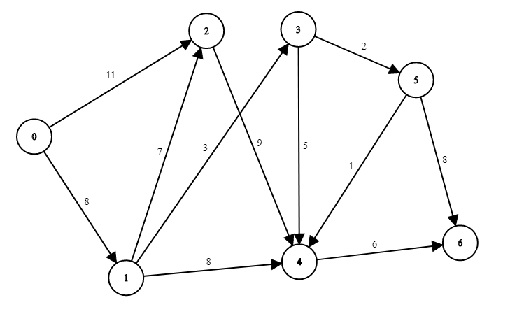
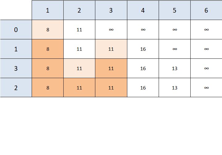
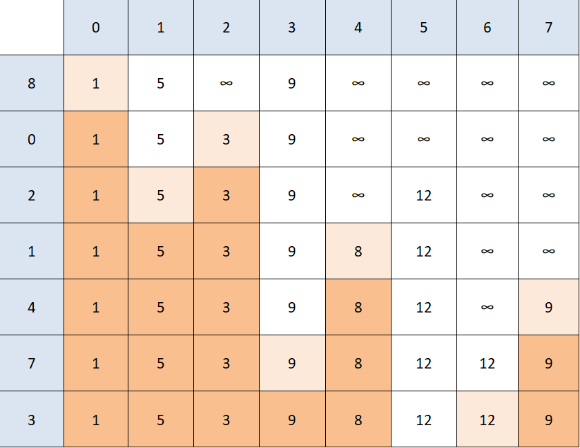
We're looking for the path with the least weight from node 0 to node 6. We will use a matrix/table to better represent what's going on in the algorithm.
At the beginning, all the data we have is the distance between 0 and its neighboring nodes.
The rest of the distances are denoted as positive infinity, i.e. they are not reachable from any of the nodes we've processed so far (we've only processed 0).
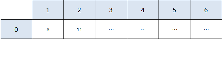
The next step is to find the closest node that hasn't been visited yet that we can actually reach from one of the nodes we've processed. In our case, this is node 1.
Now we'll update the shortest path values if it's necessary. For example, node 3 is now reachable from node 1.
We'll also mark 1 as visited.
Note: We have to take into account how much it "costs" to get to node 1. Since our starting position is 0 and it costs 8 units to get from 0 to 1, we have to add that 8 to the total cost from "moving" from 1 to another node. This is why we add 8 (distance from 0 to 1) + 3 (distance from 1 to 3) = 11 to our table, instead of just 3.
We see that from node 1 we can reach nodes 2, 3, and 4.
- Node 2 -> to get from 1 to 2 costs 7 units, given that the shortest path from 0 to 1 costs 8 units, 8 + 7 is greater than 11 (the shortest path between 0 and 2). This means we haven't found a better path from 0 to 2 through the node 1, so we don't change anything.
- Node 3 -> to get from 1 to 3 costs 3 units, and since 3 was previously unreachable, 8 + 3 is definitely better than positive infinity, so we update the table in that cell
- Node 4 -> same as with node 3, previously unreachable so we update the table for node 4 as well
The dark orange shading helps us keep track of nodes we have visited, we'll discuss why the lighter orange shade was added later.
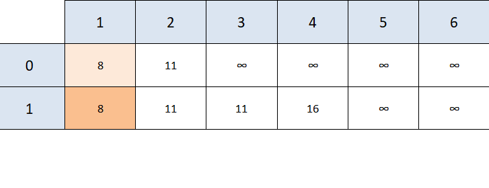
We can now choose between node 2 and node 3, since both are as "close" to node 0. Let's go with node 3.
Unvisited, reachable nodes from node 3 are nodes 4 and 5:
- Node 4 -> it costs 5 units to get from node 3 to node 4, and 11 + 5 isn't better than the previous 16 unit value we found, so there's no need to update
- Node 5 -> it costs 2 units to get from node 3 to node 5, and 11 + 2 is better than positive infinity, so we update the table
- We mark 3 as visited.
The next node to consider is node 2, however the only node reachable from node 2 is node 4 and the value we get (11 + 9 = 20) isn't better than the previous value we found (16), so we make no changes to our table, other than mark node 2 as visited.
The next closest reachable node is 5, and 5's unvisited neighbors are 4 and 6.
- Node 4 -> 13 + 1 is better than 16, so the value is updated
- Node 6 -> 13 + 8 is better than positive infinity, so the value is updated
- Mark 5 as visited.
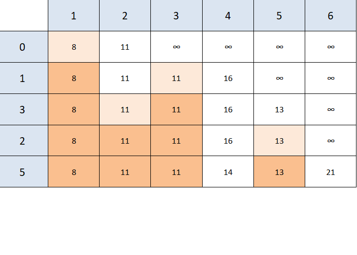
Even though we can reach the end node, that's not the closest reachable node (4 is), so we need to visit 4 to check whether it has a better path to node 6.
It turns out that it does. 6 is the only unvisited node reachable from node 4, and 14 + 6 is less than 21. So we updated our table one last time.
Since the next closest, reachable, unvisited node is our end node - the algorithm is over and we have our result - the value of the shortest path between 0 and 6 is 20.
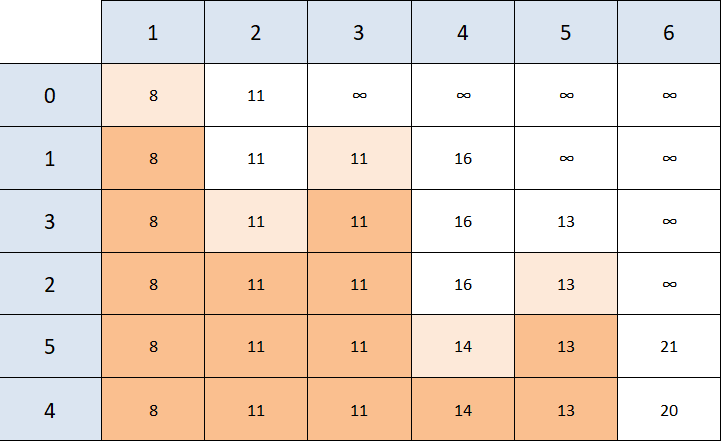
This, however, doesn't give us the answer to "WHAT is the cheapest path" between 0 and 6, it only tells us its value. This is where the light orange shading comes in.
We need to figure out how we got to 6, and we do this by checking "when did the value of the shortest path to 6 change the last time?".
Looking at our table, we can see that the value changed from 21 to 20 when we were looking at node 4. We can either see that by looking at the row name that we were in when the value became 20, or the light orange cell's column name right before the value changed.
Now we know that we've arrived at node 6 from node 4, but how did we get to node 4? Following the same principle - we see that 4's value changed for the last time when we were looking at node 5.
Applying the same principle to node 5 -> we arrived from node 3; we arrived at node 3 from node 1, and to node 1 from our starting node, node 0.
This gives us the path 0 -> 1 -> 3 -> 5 -> 4 -> 6 as the path with the least value from 0 to 6. This path sometimes isn't unique, there can be several paths that have the same value.
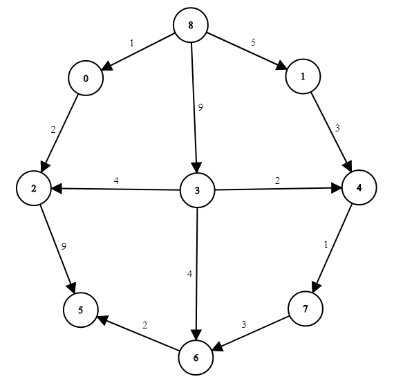
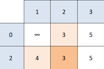
If you wish to practice the algorithm on another graph before we go into the code, here's another example and the solution - try to find the solution on your own first. We'll be looking for the shortest path between 8 and 6:
Note: Dijkstra's algorithm doesn't work on every type of graph. You might have noticed that we haven't used any negative weights on our edges in our examples - this is because of the simple reason that Dijkstra doesn't work on graphs with any negative weights.
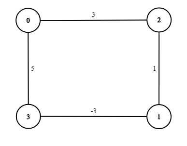
If we ran the algorithm, looking for the least expensive path between 0 and 1, the algorithm would return 0 -> 2 -> 1 even though that's not correct (the least expensive path is 0 -> 3 -> 1).
Dijkstra's algorithm sees that the next closest node is 1 so it doesn't check the rest of the unvisited nodes. This just goes to show that Dijkstra doesn't work with graphs that contain negative edges.
Now onto the interesting part - the actual code. There are several ways to design classes for this algorithm, but we've chosen to keep the list of EdgeWeighted objects in the NodeWeighted class, so we have easy access to all the edges from a particular node.
Also, every EdgeWeighted object contains the source NodeWeighted object and the destination NodeWeighted object, just in case we want to try and implement the algorithm differently in the future.
Note: Our implementation relies on objects equality in the true sense, and all our methods share the exact same NodeWeighted object, so any change to that object reflects on the entire graph. This might not be something you want in your code, however relying on this makes our code much more readable and better for educational purposes, so we've chosen that approach.
Implementing a Weighted Graph
Let's start off with the simplest class of all we'll use, the EdgeWeighted class:
Check out our hands-on, practical guide to learning Git, with best-practices, industry-accepted standards, and included cheat sheet. Stop Googling Git commands and actually learn it!
public class EdgeWeighted implements Comparable<EdgeWeighted> {

    NodeWeighted source;
    NodeWeighted destination;
    double weight;

    EdgeWeighted(NodeWeighted s, NodeWeighted d, double w) {
        // Note that we are choosing to use the (exact) same objects in the Edge class
        // and in the GraphShow and GraphWeighted classes on purpose - this MIGHT NOT
        // be something you want to do in your own code, but for sake of readability
        // we've decided to go with this option
        source = s;
        destination = d;
        weight = w;
    }

    // ...
}
The NodeWeighted objects represent the actual nodes in our weighted graph. We'll implement that class shortly after the edges.
Now, let's simply implement the toString() method for the sake of printing objects and the compareTo() method:
public String toString() {
    return String.format("(%s -> %s, %f)", source.name, destination.name, weight);
}

// We need this method if we want to use PriorityQueues instead of LinkedLists
// to store our edges, the benefits are discussed later, we'll be using LinkedLists
// to make things as simple as possible
public int compareTo(EdgeWeighted otherEdge) {

    // We can't simply use return (int)(this.weight - otherEdge.weight) because
    // this sometimes gives false results
    if (this.weight > otherEdge.weight) {
        return 1;
    }
    else return -1;
}
With our weighted edges out of the way, let's implement our weighted nodes:
public class NodeWeighted {
    // The int n and String name are just arbitrary attributes
    // we've chosen for our nodes these attributes can of course
    // be whatever you need
    int n;
    String name;
    private boolean visited;
    LinkedList<EdgeWeighted> edges;

    NodeWeighted(int n, String name) {
        this.n = n;
        this.name = name;
        visited = false;
        edges = new LinkedList<>();
    }

    boolean isVisited() {
        return visited;
    }

    void visit() {
        visited = true;
    }

    void unvisit() {
        visited = false;
    }
}
The NodeWeighted is a pretty straightforward class resembling regular nodes we've used before. This time around, the Graph class isn't the one holding the information about the edges between the nodes, but rather, each node contains a list of its own neighbors.
Finally, let's implement the GraphWeighted class which will utilize both of the previous classes to represent a graph:
public class GraphWeighted {
    private Set<NodeWeighted> nodes;
    private boolean directed;

    GraphWeighted(boolean directed) {
        this.directed = directed;
        nodes = new HashSet<>();
    }

    // ...
}
To store our nodes in the graph, we'll be using a Set. They're convenient for us since they don't allow duplicate objects and are generally simple to work with.
Now, as usual, let's define the main methods we'll use to build our graph, starting off with the addNode() method:
// Doesn't need to be called for any node that has an edge to another node
// since addEdge makes sure that both nodes are in the nodes Set
public void addNode(NodeWeighted... n) {
    // We're using a var arg method so we don't have to call
    // addNode repeatedly
    nodes.addAll(Arrays.asList(n));
}
And with it, the addEdge() method alongside the addEdgeHelper() method used for convenience and readability:
public void addEdge(NodeWeighted source, NodeWeighted destination, double weight) {
    // Since we're using a Set, it will only add the nodes
    // if they don't already exist in our graph
    nodes.add(source);
    nodes.add(destination);

    // We're using addEdgeHelper to make sure we don't have duplicate edges
    addEdgeHelper(source, destination, weight);

    if (!directed && source != destination) {
        addEdgeHelper(destination, source, weight);
    }
}

private void addEdgeHelper(NodeWeighted a, NodeWeighted b, double weight) {
    // Go through all the edges and see whether that edge has
    // already been added
    for (EdgeWeighted edge : a.edges) {
        if (edge.source == a && edge.destination == b) {
            // Update the value in case it's a different one now
            edge.weight = weight;
            return;
        }
    }
    // If it hasn't been added already (we haven't returned
    // from the for loop), add the edge
    a.edges.add(new EdgeWeighted(a, b, weight));
}
At this point, our main logic for the GraphWeighted is done. We simply need some method to print edges, check if there's an edge between two nodes and reset all visited nodes.
Let's start off with printing edges:
public void printEdges() {
    for (NodeWeighted node : nodes) {
        LinkedList<EdgeWeighted> edges = node.edges;

        if (edges.isEmpty()) {
            System.out.println("Node " + node.name + " has no edges.");
            continue;
        }
        System.out.print("Node " + node.name + " has edges to: ");

        for (EdgeWeighted edge : edges) {
            System.out.print(edge.destination.name + "(" + edge.weight + ") ");
        }
        System.out.println();
    }
}
Now, a simple check if two nodes have an edge between them:
public boolean hasEdge(NodeWeighted source, NodeWeighted destination) {
    LinkedList<EdgeWeighted> edges = source.edges;
    for (EdgeWeighted edge : edges) {
        // Again relying on the fact that all classes share the
        // exact same NodeWeighted object
        if (edge.destination == destination) {
            return true;
        }
    }
    return false;
}
And finally, the method that resets all visited nodes so we can practically reset the algorithm:
// Necessary call if we want to run the algorithm multiple times
public void resetNodesVisited() {
    for (NodeWeighted node : nodes) {
        node.unvisit();
    }
}
Implementing Dijkstra's Algorithm
With our weighted graph and nodes all done, we can finally focus on Dijkstra's Algorithm itself. It's going to be a bit long with many explanations in the comments, so bear with us for a moment:
public void DijkstraShortestPath(NodeWeighted start, NodeWeighted end) {
    // We keep track of which path gives us the shortest path for each node
    // by keeping track how we arrived at a particular node, we effectively
    // keep a "pointer" to the parent node of each node, and we follow that
    // path to the start
    HashMap<NodeWeighted, NodeWeighted> changedAt = new HashMap<>();
    changedAt.put(start, null);

    // Keeps track of the shortest path we've found so far for every node
    HashMap<NodeWeighted, Double> shortestPathMap = new HashMap<>();

    // Setting every node's shortest path weight to positive infinity to start
    // except the starting node, whose shortest path weight is 0
    for (NodeWeighted node : nodes) {
        if (node == start)
            shortestPathMap.put(start, 0.0);
        else shortestPathMap.put(node, Double.POSITIVE_INFINITY);
    }

    // Now we go through all the nodes we can go to from the starting node
    // (this keeps the loop a bit simpler)
    for (EdgeWeighted edge : start.edges) {
        shortestPathMap.put(edge.destination, edge.weight);
        changedAt.put(edge.destination, start);
    }

    start.visit();

    // This loop runs as long as there is an unvisited node that we can
    // reach from any of the nodes we could till then
    while (true) {
        NodeWeighted currentNode = closestReachableUnvisited(shortestPathMap);
        // If we haven't reached the end node yet, and there isn't another
        // reachable node the path between start and end doesn't exist
        // (they aren't connected)
        if (currentNode == null) {
            System.out.println("There isn't a path between " + start.name + " and " + end.name);
            return;
        }

        // If the closest non-visited node is our destination, we want to print the path
        if (currentNode == end) {
            System.out.println("The path with the smallest weight between "
                                   + start.name + " and " + end.name + " is:");

            NodeWeighted child = end;

            // It makes no sense to use StringBuilder, since
            // repeatedly adding to the beginning of the string
            // defeats the purpose of using StringBuilder
            String path = end.name;
            while (true) {
                NodeWeighted parent = changedAt.get(child);
                if (parent == null) {
                    break;
                }

                // Since our changedAt map keeps track of child -> parent relations
                // in order to print the path we need to add the parent before the child and
                // it's descendants
                path = parent.name + " " + path;
                child = parent;
            }
            System.out.println(path);
            System.out.println("The path costs: " + shortestPathMap.get(end));
            return;
        }
        currentNode.visit();

        // Now we go through all the unvisited nodes our current node has an edge to
        // and check whether its shortest path value is better when going through our
        // current node than whatever we had before
        for (EdgeWeighted edge : currentNode.edges) {
            if (edge.destination.isVisited())
                continue;

            if (shortestPathMap.get(currentNode)
               + edge.weight
               < shortestPathMap.get(edge.destination)) {
                shortestPathMap.put(edge.destination,
                                   shortestPathMap.get(currentNode) + edge.weight);
                changedAt.put(edge.destination, currentNode);
            }
        }
    }
}
And finally, let's define the closestReachableUnvisited() method that evaluates which is the closest node that we can reach and haven't visited before:
private NodeWeighted closestReachableUnvisited(HashMap<NodeWeighted, Double> shortestPathMap) {

    double shortestDistance = Double.POSITIVE_INFINITY;
    NodeWeighted closestReachableNode = null;
    for (NodeWeighted node : nodes) {
        if (node.isVisited())
            continue;

        double currentDistance = shortestPathMap.get(node);
        if (currentDistance == Double.POSITIVE_INFINITY)
            continue;

        if (currentDistance < shortestDistance) {
            shortestDistance = currentDistance;
            closestReachableNode = node;
        }
    }
    return closestReachableNode;
}
Now that we have all that - let's test our algorithm on the first example from above:
public class GraphShow {
    public static void main(String[] args) {
        GraphWeighted graphWeighted = new GraphWeighted(true);
        NodeWeighted zero = new NodeWeighted(0, "0");
        NodeWeighted one = new NodeWeighted(1, "1");
        NodeWeighted two = new NodeWeighted(2, "2");
        NodeWeighted three = new NodeWeighted(3, "3");
        NodeWeighted four = new NodeWeighted(4, "4");
        NodeWeighted five = new NodeWeighted(5, "5");
        NodeWeighted six = new NodeWeighted(6, "6");

        // Our addEdge method automatically adds Nodes as well.
        // The addNode method is only there for unconnected Nodes,
        // if we wish to add any
        graphWeighted.addEdge(zero, one, 8);
        graphWeighted.addEdge(zero, two, 11);
        graphWeighted.addEdge(one, three, 3);
        graphWeighted.addEdge(one, four, 8);
        graphWeighted.addEdge(one, two, 7);
        graphWeighted.addEdge(two, four, 9);
        graphWeighted.addEdge(three, four, 5);
        graphWeighted.addEdge(three, five, 2);
        graphWeighted.addEdge(four, six, 6);
        graphWeighted.addEdge(five, four, 1);
        graphWeighted.addEdge(five, six, 8);

        graphWeighted.DijkstraShortestPath(zero, six);
    }
}
We get the following output:
The path with the smallest weight between 0 and 6 is:
0 1 3 5 4 6
The path costs: 20.0
Which is exactly what we got by manually doing the algorithm.
Using it on the second example from above gives us the following output:
The path with the smallest weight between 8 and 6 is:
8 1 4 7 6
The path costs: 12.0
Furthermore, while searching for the cheapest path between two nodes using Dijkstra, we most likely found multiple other cheapest paths between our starting node and other nodes in the graph. Actually - we've found the cheapest path from source to node for every visited node. Just sit on that for a moment, we'll prove this in a latter section.
However, if we wanted to know the shortest path between our starting node and all other nodes we would need to keep running the algorithm on all nodes that aren't visited yet. In the worst case scenario we'd need to run the algorithm numberOfNodes - 1 times.
Note: Dijkstra's algorithm is an example of a greedy algorithm. Meaning that at every step, the algorithm does what seems best at that step, and doesn't visit a node more than once. Such a step is locally optimal but not necessarily optimal in the end.
This is why Dijkstra fails with negatively weighted edges, it doesn't revisit nodes that might have a cheaper path through a negatively weighted edge because the node has already been visited. However - without negatively weighted edges, Dijkstra is globally optimal (i.e. it works).
Dijkstra's Complexity
Let's consider the complexity of this algorithm, and look at why we mentioned PriorityQueue and added a compareTo() method to our EdgeWeighted class.
The bottleneck of Dijkstra's algorithm is finding the next closest, unvisited node/vertex. Using LinkedList this has a complexity of O(numberOfEdges), since in the worst case scenario we need to go through all the edges of the node to find the one with the smallest weight.
To make this better, we can use Java's heap data structure - PriorityQueue. Using a PriorityQueue guarantees us that the next closest, unvisited node (if there is one) will be the first element of the PriorityQueue.
So - now finding the next closest node is done in constant (O(1)) time, however, keeping the PriorityQueue sorted (removing used edges and adding new ones) takes O(log(numberOfEdges)) time. This is still much better than O(numberOfEdges).
Further, we have O(numberOfNodes) iterations and therefore as many deletions from the PriorityQueue (that take O(log(numberOfEdges)) time), and adding all of our edges also takes O(log(numberOfEdges)) time.
This gives us a total of O((numberOfEdges + numberOfNodes) * log(numberOfEdges)) complexity when using PriorityQueue.
If we didn't use PriorityQueue (like we didn't) - the complexity would be O((numberOfEdges + numberOfNodes) * numberOfEdges) .
Correctness of Dijkstra's Algorithm
So far we've been using Dijkstra's algorithm without really proving that it actually works. The algorithm is "intuitive" enough for us to take that fact for granted but let's prove that that is actually the case.
We'll use mathematical induction to prove the correctness of this algorithm.
What does "correctness" mean in our case?
Well - we want to prove that at the end of our algorithm, all the paths we've found (all the nodes we've visited) are actually the cheapest paths from the source to that node, including the destination node when we get to it.
We prove this by proving that it's true at the start (for the start node) and we prove that it keeps being true at every step of the algorithm.
Let's define some shorthand names for things we'll need in this proof:
CPF(x): Cheapest Path Found from start node to node xACP(x): Actual Cheapest Path from start node to node xd(x,y): The distance/weight of the edge between nodes y and xV: All the nodes visited so far
Alright, so we want to prove that at every step of the algorithm, and at the end x ∈ V, CPF(x) = ACP(x), i.e. that for every node we've visited, the cheapest path we've found is actually the cheapest path for that node.
Base Case: (at the beginning) we have only one node in V, and that is the starting node. So since V = {start} and ACP(start) = 0 = CPF(start), our algorithm is correct.
Inductive Hypothesis: After adding a node n to V (visiting that node), for every x ∈ V => CPF(x) = ACP(x)
Inductive Step: We know that for V without n our algorithm is correct. We need to prove that it stays correct after adding a new node n. Let's say that V' is V ∪ {n} (in other words, V' is what we get after visiting node n).
So we know that for every node in V our algorithm is correct, i.e. that for every x ∈ V, CPF(x) => ACP(x), so to make it true for V' we need to prove that CPF(n) = ACP(n).
We'll prove this by contradiction, that is we'll assume that CPF(n) ≠ ACP(n) and show that that isn't possible.
Let's assume that ACP(n) < CPF(n).
The ACP(n) starts somewhere in V and at some point leaves V to get to n (since n isn't in V, it has to leave V). Let's say that some edge (x,y) is the first edge that leaves V, i.e. that x is in V but y isn't.
We know two things:
- The path that got us the
ACP(x)is a subpath of the path that gets usACP(n) ACP(x) + d(x,y) <= ACP(n)(since there are at least as many nodes between start andyas there are between start andn, since we know the cheapest path tongoes throughy)
Our inductive hypothesis says that CPF(x) = ACP(x) which lets us change (2) to CPF(x) + d(x,y) <= ACP(x).
Since y is adjacent to x, the algorithm must have updated the value of y when looking at x (since x is in V), so we know that CPF(y) <= CPF(x) + d(x,y).
Also since the node n was picked by the algorithm we know that n must be the closest node of all the unvisited (reminder: y was also unvisited and was supposed to be on the shortest path to n), which means that CPF(n) <= CPF(y).
If we combine all these inequalities we'll see that CPF(n) < ACP(n) which gives us a contradiction i.e. our assumption that ACP(n) < CPF(n) wasn't correct.
CPF(n) <= CPF(y)andCPF(y) <= CPF(x) + d(x,y)give us ->CPF(n) <= CPF(x) + d(x,y)CPF(x) + d(x,y) <= ACP(x)andACP(x) + d(x,y) <= ACP(n)give us ->CPF(n) <= ACP(x)which then gives usCPF(n) < ACP(n)
Therefore our algorithm does what it's supposed to.
Note: This also proves that the paths to all the nodes we've visited during the algorithm are also the cheapest paths to those nodes, not just the path we found for the destination node.
Conclusion
Graphs are a convenient way to store certain types of data. The concept was ported from mathematics and appropriated for the needs of computer science. Due to the fact that many things can be represented as graphs, graph traversal has become a common task, especially used in data science and machine learning.
Dijkstra's algorithm finds the least expensive path in a weighted graph between our starting node and a destination node, if such a path exists. It starts at the destination node and backtracks its way back to the root node, along the weighted edges in the "cheapest" path to cross.

