Introduction to Neural Networks with Scikit-Learn

What is a Neural Network?

Humans have an ability to identify patterns within the accessible information with an astonishingly high degree of accuracy. Whenever you see a car or a bicycle you can immediately recognize what they are. This is because we have learned over a period of time how a car and bicycle looks like and what their distinguishing features are. Artificial neural networks are computation systems that intend to imitate human learning capabilities via a complex architecture that resembles the human nervous system.

In this article, we will just briefly review what neural networks are, what are the computational steps that a neural network goes through (without going down into the complex mathematics behind it), and how they can be implemented using Scikit-Learn, which is a popular AI library for Python.

The Human Nervous System

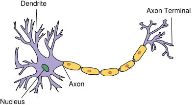
Human nervous system consists of billions of neurons. These neurons collectively process input received from sensory organs, process the information, and decide what to do in reaction to the input. A typical neuron in the human nervous system has three main parts: dendrites, nucleus, and axons. The information passed to a neuron is received by dendrites. The nucleus is responsible for processing this information. The output of a neuron is passed to other neurons via the axon, which is connected to the dendrites of other neurons further down the network.

Perceptrons

Artificial neural networks are inspired by the human neural network architecture. The simplest neural network consists of only one neuron and is called a perceptron, as shown in the figure below:

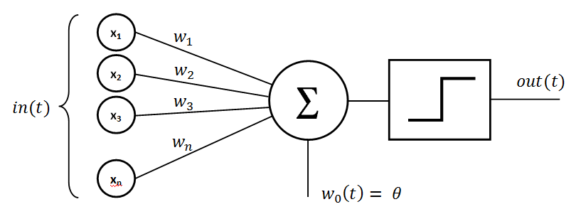
A perceptron has one input layer and one neuron. Input layer acts as the dendrites and is responsible for receiving the inputs. The number of nodes in the input layer is equal to the number of features in the input dataset. Each input is multiplied with a weight (which is typically initialized with some random value) and the results are added together. The sum is then passed through an activation function. The activation function of a perceptron resembles the nucleus of the human nervous system neuron. It processes the information and yields an output. In the case of a perceptron, this output is the final outcome. However, in the case of multilayer perceptrons, the output from the neurons in the previous layer serves as the input to the neurons of the proceeding layer.

Artificial Neural Network (Multilayer Perceptron)

Now that we know what a single layer perceptron is, we can extend this discussion to multilayer perceptrons, or more commonly known as artificial neural networks. A single layer perceptron can solve simple problems where data is linearly separable into 'n' dimensions, where 'n' is the number of features in the dataset. However, in case of non-linearly separable data, the accuracy of single layer perceptrons decreases significantly. Multilayer perceptrons, on the other hand, can work efficiently with non-linearly separable data.

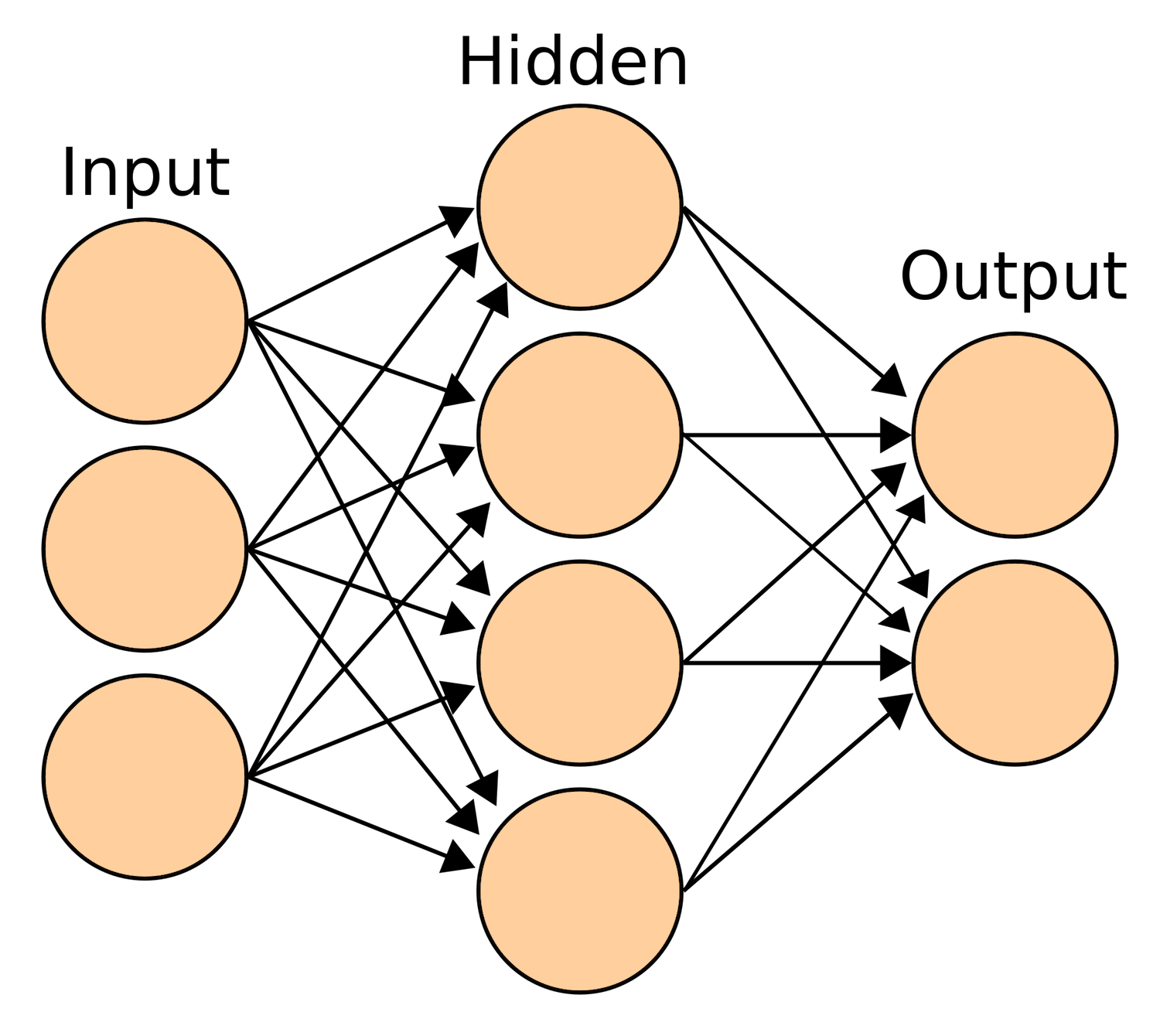
Multilayer perceptrons, or more commonly referred to as artificial neural networks, are a combination of multiple neurons connected in the form of a network. An artificial neural network has an input layer, one or more hidden layers, and an output layer. This is shown in the image below:

A neural network executes in two phases: Feed-Forward and Back Propagation.

Feed-Forward

Following are the steps performed during the feed-forward phase:

1. The values received in the input layer are multiplied with the weights. A bias is added to the summation of the inputs and weights in order to avoid null values.
2. Each neuron in the first hidden layer receives different values from the input layer depending upon the weights and bias. Neurons have an activation function that operates upon the value received from the input layer. The activation function can be of many types, like a step function, sigmoid function, relu function, or tanh function. As a rule of thumb, ReLU function is used in the hidden layer neurons and sigmoid function is used for the output layer neuron.
3. The outputs from the first hidden layer neurons are multiplied with the weights of the second hidden layer; the results are summed together and passed to the neurons of the proceeding layers. This process continues until the outer layer is reached. The values calculated at the outer layer are the actual outputs of the algorithm.

The feed-forward phase consists of these three steps. However, the predicted output is not necessarily correct right away; it can be wrong, and we need to correct it. The purpose of a learning algorithm is to make predictions that are as accurate as possible. To improve these predicted results, a neural network will then go through a back propagation phase. During back propagation, the weights of different neurons are updated in a way that the difference between the desired and predicted output is as small as possible.

Back Propagation

Back propagation phase consists of the following steps:

1. The error is calculated by quantifying the difference between the predicted output and the desired output. This difference is called "loss" and the function used to calculate the difference is called the "loss function". Loss functions can be of different types e.g. mean squared error or cross entropy functions. Remember, neural networks are supervised learning algorithms that need the desired outputs for a given set of inputs, which is what allows it to learn from the data.
2. Once the error is calculated, the next step is to minimize that error. To do so, the partial derivative of the error function is calculated with respect to all the weights and biases. This is called gradient descent. The derivatives can be used to find the slope of the error function. If the slope is positive, the value of the weights can be reduced or if the slope is negative the value of weight can be increased. This reduces the overall error. The function that is used to reduce this error is called the optimization function.

This one cycle of feed-forward and back propagation is called one "epoch". This process continues until a reasonable accuracy is achieved. There is no standard for reasonable accuracy, ideally you'd strive for 100% accuracy, but this is extremely difficult to achieve for any non-trivial dataset. In many cases 90%+ accuracy is considered acceptable, but it really depends on your use-case.

Implementing Neural Network with Scikit-Learn

Now we know what neural networks are and what are the different steps that we need to perform in order to build a simple, densely connected neural network. In this section we will try to build a simple neural network that predicts the class that a given iris plant belongs to. We will use Python's Scikit-Learn library to create our neural network that performs this classification task. The download and installation instructions for the Scikit-Learn library are available at: http://scikit-learn.org/stable/install.html

Note: The scripts provided with this tutorial have been executed and tested in a Python Jupyter notebook.

Dataset

The dataset that we are going to use for this tutorial is the popular Iris dataset, available at https://archive.ics.uci.edu/ml/datasets/iris. The details of the dataset are available at the aforementioned link.

Let's jump straight to the code. The first step is to import this dataset into our program. To do so, we will use Python's pandas library.

Execute the following command to load the iris dataset into a Python dataframe:

import pandas as pd

# Location of dataset
url = "https://archive.ics.uci.edu/ml/machine-learning-databases/iris/iris.data"

# Assign column names to the dataset
names = ['sepal-length', 'sepal-width', 'petal-length', 'petal-width', 'Class']

# Read dataset to pandas dataframe
irisdata = pd.read_csv(url, names=names)

The above script simply downloads the iris data, assigns the names i.e. sepal-length, sepal-width, petal-length, petal-width, and Class to the columns of the dataset, and then loads it into the irisdata data frame.

To see what this dataset actually looks like, execute the following command:

irisdata.head()

Executing the above script will display the first five rows of our dataset, as shown below:

	sepal-length	sepal-width	petal-length	petal-width	Class
0	5.1	3.5	1.4	0.2	Iris-setosa
1	4.9	3.0	1.4	0.2	Iris-setosa
2	4.7	3.2	1.3	0.2	Iris-setosa
3	4.6	3.1	1.5	0.2	Iris-setosa
4	5.0	3.6	1.4	0.2	Iris-setosa

Preprocessing

You can see that our dataset has five columns. The task is to predict the class (which are the values in the fifth column) that the iris plant belongs to, which is based upon the sepal-length, sepal-width, petal-length and petal-width (the first four columns). The next step is to split our dataset into attributes and labels. Execute the following script to do so:

# Assign data from first four columns to X variable
X = irisdata.iloc[:, 0:4]

# Assign data from first fifth columns to y variable
y = irisdata.select_dtypes(include=[object])

To see what y looks like, execute the following code:

y.head()

	Class
0	Iris-setosa
1	Iris-setosa
2	Iris-setosa
3	Iris-setosa
4	Iris-setosa

You can see that the values in the y series are categorical. However, neural networks work better with numerical data. Our next task is to convert these categorical values to numerical values. But first let's see how many unique values we have in our y series. Execute the following script:

y.Class.unique()

Output:

array(['Iris-setosa', 'Iris-versicolor', 'Iris-virginica'], dtype=object)

We have three unique classes: 'Iris-setosa', 'Iris-versicolor' and 'Iris-virginica'. Let's convert these categorical values to numerical values. To do so we will use Scikit-Learn's LabelEncoder class.

Execute the following script:

from sklearn import preprocessing
le = preprocessing.LabelEncoder()

y = y.apply(le.fit_transform)

Now if you again check unique values in the y series, you will see following results:

array([0, 1, 2], dtype=int64)

You can see that the categorical values have been encoded to numerical values i.e. 0, 1, and 2.

Train Test Split

To avoid over-fitting, we will divide our dataset into training and test splits. The training data will be used to train the neural network and the test data will be used to evaluate the performance of the neural network. This helps with the problem of over-fitting because we're evaluating our neural network on data that it has not seen (i.e. been trained on) before.

To create training and test splits, execute the following script:

from sklearn.model_selection import train_test_split
X_train, X_test, y_train, y_test = train_test_split(X, y, test_size = 0.20)

The above script splits 80% of the dataset into our training set and the other 20% into test data.

Feature Scaling

Before making actual predictions, it is always a good practice to scale the features so that all of them can be uniformly evaluated. Feature scaling is performed only on the training data and not on test data. This is because in the real world, data is not scaled and the ultimate purpose of the neural network is to make predictions on real world data. Therefore, we try to keep our test data as real as possible.

The following script performs feature scaling:

from sklearn.preprocessing import StandardScaler
scaler = StandardScaler()
scaler.fit(X_train)

X_train = scaler.transform(X_train)
X_test = scaler.transform(X_test)

Training and Predictions

And now it's finally time to do what you have been waiting for, train a neural network that can actually make predictions. To do this, execute the following script:

from sklearn.neural_network import MLPClassifier
mlp = MLPClassifier(hidden_layer_sizes=(10, 10, 10), max_iter=1000)
mlp.fit(X_train, y_train.values.ravel())

Yes, with Scikit-Learn, you can create a neural network with these three lines of code, which all handles much of the leg work for you. Let's see what is happening in the above script. The first step is to import the MLPClassifier class from the sklearn.neural_network library. In the second line, this class is initialized with two parameters.

The first parameter, hidden_layer_sizes, is used to set the size of the hidden layers. In our script we will create three layers of 10 nodes each. There is no standard formula for choosing the number of layers and nodes for a neural network and it varies quite a bit depending on the problem at hand. The best way is to try different combinations and see what works best.

The second parameter to MLPClassifier specifies the number of iterations, or the epochs, that you want your neural network to execute. Remember, one epoch is a combination of one cycle of feed-forward and back propagation phase.

By default the 'ReLU' activation function is used with adam cost optimizer. However, you can change these functions using the activation and solver parameters, respectively.

In the third line the fit function is used to train the algorithm on our training data i.e. X_train and y_train.

The final step is to make predictions on our test data. To do so, execute the following script:

predictions = mlp.predict(X_test)

Evaluating the Algorithm

We created our algorithm and we made some predictions on the test dataset. Now is the time to evaluate how well our algorithm performs. To evaluate an algorithm, the most commonly used metrics are a confusion matrix, precision, recall, and f1 score. The confusion_matrix and classification_report methods of the sklearn.metrics library can help us find these scores. The following script generates evaluation report for our algorithm:

from sklearn.metrics import classification_report, confusion_matrix
print(confusion_matrix(y_test,predictions))
print(classification_report(y_test,predictions))

This code above generates the following result:

[[11  0  0]
   0  8  0]
   0  1 10]]
             precision   recall   f1-score   support
          0       1.00     1.00       1.00        11
          1       0.89     1.00       0.94         8
          2       1.00     0.91       0.95        11

avg / total       0.97     0.97       0.97        30

You can see from the confusion matrix that our neural network only misclassified one plant out of the 30 plants we tested the network on. Also, the f1 score of 0.97 is very good, given the fact that we only had 150 instances to train.

Your results can be slightly different from these because train_test_split randomly splits data into training and test sets, so our networks may not have been trained/tested on the same data. But overall, the accuracy should be greater than 90% on your datasets as well.

Conclusion

In this article we gave a brief overview of what neural networks are and we explained how to create a very simple neural network that was trained on the iris dataset. I would recommend you try to play around with the number of hidden layers, activation functions, and size of the training and testing split to see if you can achieve better results than what we presented here.