Introduction to PyTorch for Classification

PyTorch and TensorFlow libraries are two of the most commonly used Python libraries for deep learning. PyTorch is developed by Facebook, while TensorFlow is a Google project. In this article, you will see how the PyTorch library can be used to solve classification problems.

Classification problems belong to the category of machine learning problems where given a set of features, the task is to predict a discrete value. Predicting whether a tumor is cancerous or not, or whether a student is likely to pass or fail in the exam, are some of the common examples of classification problems.

In this article, given certain characteristics of a bank customer, we will predict whether or not the customer is likely to leave the bank after 6 months. The phenomenon where a customer leaves an organization is also called customer churn. Therefore, our task is to predict customer churn based on various customer characteristics.

Before you proceed, it is assumed that you have intermediate level proficiency with the Python programming language and you have installed the PyTorch library. Also, know-how of basic machine learning concepts may help. If you have not installed PyTorch, you can do so with the following pip command:

$ pip install pytorch

The Dataset

The dataset that we are going to use in this article is freely available at this Kaggle link. Let's import the required libraries, and the dataset into our Python application:

import torch
import torch.nn as nn
import numpy as np
import pandas as pd
import matplotlib.pyplot as plt
import seaborn as sns
%matplotlib inline

We can use the read_csv() method of the pandas library to import the CSV file that contains our dataset.

dataset = pd.read_csv(r'E:Datasets\customer_data.csv')

Let's print the shape of our dataset:

dataset.shape

Output:

(10000, 14)

The output shows that the dataset has 10 thousand records and 14 columns.

We can use the head() method of the pandas dataframe to print the first five rows of our dataset.

dataset.head()

Output:

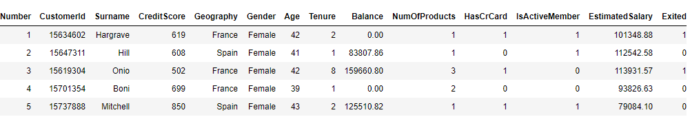
You can see the 14 columns in our dataset. Based on the first 13 columns, our task is to predict the value for the 14th column i.e. Exited. It is important to mention that the values for the first 13 columns are recorded 6 months before the value for the Exited column was obtained since the task is to predict customer churn after 6 months from the time when the customer information is recorded.

Exploratory Data Analysis

Let's perform some exploratory data analysis on our dataset. We'll first predict the ratio of the customer who actually left the bank after 6 months and will use a pie plot to visualize.

Let's first increase the default plot size for the graphs:

fig_size = plt.rcParams["figure.figsize"]
fig_size[0] = 10
fig_size[1] = 8
plt.rcParams["figure.figsize"] = fig_size

The following script draws the pie plot for the Exited column.

dataset.Exited.value_counts().plot(kind='pie', autopct='%1.0f%%', colors=['skyblue', 'orange'], explode=(0.05, 0.05))

Output:

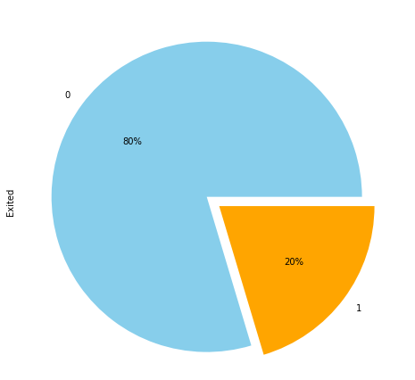
The output shows that in our dataset, 20% of the customers left the bank. Here 1 belongs to the case where the customer left the bank, where 0 refers to the scenario where a customer didn't leave the bank.

Let's plot the number of customers from all the geographical locations in the dataset:

sns.countplot(x='Geography', data=dataset)

Output:

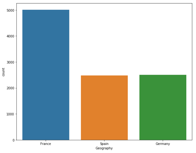
The output shows that almost half of the customers belong to France, while the ratio of customers belonging to Spain and Germany is 25% each.

Let's now plot the number of customers from each unique geographical location along with customer churn information. We can use the countplot() function from the seaborn library to do so.

sns.countplot(x='Exited', hue='Geography', data=dataset)

Output:

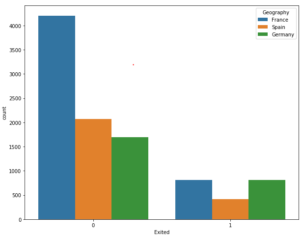
The output shows that though the overall number of French customers is twice that of the number of Spanish and German customers, the ratio of customers who left the bank is the same for French and German customers. Similarly, the overall number of German and Spanish customers is the same, but the number of German customers who left the bank is twice that of the Spanish customers, which shows that German customers are more likely to leave the bank after 6 months.

In this article, we will not visually plot the information related to the rest of the columns in our dataset, but if you want to do so, you check my article on how to perform exploratory data analysis with Python Seaborn Library.

Data Preprocessing

Before we train our PyTorch model, we need to preprocess our data. If you look at the dataset, you will see that it has two types of columns: Numerical and Categorical. The numerical columns contain numerical information. CreditScore, Balance, Age, etc. Similarly, Geography and Gender are categorical columns since they contain categorical information such as the locations and genders of the customers. There are a few columns that can be treated as numeric as well as categorical. For instance, the HasCrCard column can have 1 or 0 as its values. However, the HasCrCard column contains information about whether or not a customer has a credit card. It is advised that the columns that can be treated as both categorical and numerical, are treated as categorical. However, it totally depends upon the domain knowledge of the dataset.

Let's again print all the columns in our dataset and find out which of the columns can be treated as numerical and which columns should be treated as categorical. The columns attribute of a dataframe prints all the column names:

dataset.columns

Output:

Index(['RowNumber', 'CustomerId', 'Surname', 'CreditScore', 'Geography',
       'Gender', 'Age', 'Tenure', 'Balance', 'NumOfProducts', 'HasCrCard',
       'IsActiveMember', 'EstimatedSalary', 'Exited'],
      dtype='object')

From the columns in our dataset, we will not use the RowNumber, CustomerId, and Surname columns since the values for these columns are totally random and have no relation with the output. For instance, a customer's surname has no impact on whether or not the customer will leave the bank. Among the rest of the columns, Geography, Gender, HasCrCard, and IsActiveMember columns can be treated as categorical columns. Let's create a list of these columns:

categorical_columns = ['Geography', 'Gender', 'HasCrCard', 'IsActiveMember']

All of the remaining columns except the Exited column can be treated as numerical columns.

numerical_columns = ['CreditScore', 'Age', 'Tenure', 'Balance', 'NumOfProducts', 'EstimatedSalary']

Finally, the output (the values from the Exited column) are stored in the outputs variable.

outputs = ['Exited']

We have created lists of categorical, numeric, and output columns. However, at the moment the type of the categorical columns is not categorical. You can check the type of all the columns in the dataset with the following script:

dataset.dtypes

Output:

RowNumber            int64
CustomerId           int64
Surname             object
CreditScore          int64
Geography           object
Gender              object
Age                  int64
Tenure               int64
Balance            float64
NumOfProducts        int64
HasCrCard            int64
IsActiveMember       int64
EstimatedSalary    float64
Exited               int64
dtype: object

You can see that the type for Geography and Gender columns is object and the type for HasCrCard and IsActive columns is int64. We need to convert the types for categorical columns to category. We can do so using the astype() function, as shown below:

for category in categorical_columns:
    dataset[category] = dataset[category].astype('category')

Now if you again plot the types for the columns in our dataset, you should see the following results:

dataset.dtypes

Output

RowNumber             int64
CustomerId            int64
Surname              object
CreditScore           int64
Geography          category
Gender             category
Age                   int64
Tenure                int64
Balance             float64
NumOfProducts         int64
HasCrCard          category
IsActiveMember     category
EstimatedSalary     float64
Exited                int64
dtype: object

Let's now see all the categories in the Geography column:

dataset['Geography'].cat.categories

Output:

Index(['France', 'Germany', 'Spain'], dtype='object')

When you change a column's data type to category, each category in the column is assigned a unique code. For instance, let's plot the first five rows of the Geography column and print the code values for the first five rows:

dataset['Geography'].head()

Output:

0    France
1     Spain
2    France
3    France
4     Spain
Name: Geography, dtype: category
Categories (3, object): [France, Germany, Spain]

The following script plots the codes for the values in the first five rows of the Geography column:

dataset['Geography'].head().cat.codes

Output:

0    0
1    2
2    0
3    0
4    2
dtype: int8

The output shows that France has been coded as 0, and Spain has been coded as 2.

The basic purpose of separating categorical columns from the numerical columns is that values in the numerical column can be directly fed into neural networks. However, the values for the categorical columns first have to be converted into numeric types. The coding of the values in the categorical column partially solves the task of numerical conversion of the categorical columns.

Since we will be using PyTorch for model training, we need to convert our categorical and numerical columns to tensors.

Let's first convert the categorical columns to tensors. In PyTorch, tensors can be created via the numpy arrays. We will first convert data in the four categorical columns into numpy arrays and then stack all the columns horizontally, as shown in the following script:

geo = dataset['Geography'].cat.codes.values
gen = dataset['Gender'].cat.codes.values
hcc = dataset['HasCrCard'].cat.codes.values
iam = dataset['IsActiveMember'].cat.codes.values

categorical_data = np.stack([geo, gen, hcc, iam], 1)

categorical_data[:10]

The above script prints the first ten records from the categorical columns, stacked horizontally. The output is as follows:

Output:

array([[0, 0, 1, 1],
       [2, 0, 0, 1],
       [0, 0, 1, 0],
       [0, 0, 0, 0],
       [2, 0, 1, 1],
       [2, 1, 1, 0],
       [0, 1, 1, 1],
       [1, 0, 1, 0],
       [0, 1, 0, 1],
       [0, 1, 1, 1]], dtype=int8)

Now to create a tensor from the aforementioned numpy array, you can simply pass the array to the tensor class of the torch module. Remember, for the categorical columns the data type should be torch.int64.

categorical_data = torch.tensor(categorical_data, dtype=torch.int64)
categorical_data[:10]

Output:

tensor([[0, 0, 1, 1],
        [2, 0, 0, 1],
        [0, 0, 1, 0],
        [0, 0, 0, 0],
        [2, 0, 1, 1],
        [2, 1, 1, 0],
        [0, 1, 1, 1],
        [1, 0, 1, 0],
        [0, 1, 0, 1],
        [0, 1, 1, 1]])

In the output, you can see that the numpy array of categorical data has now been converted into a tensor object.

In the same way, we can convert our numerical columns to tensors:

numerical_data = np.stack([dataset[col].values for col in numerical_columns], 1)
numerical_data = torch.tensor(numerical_data, dtype=torch.float)
numerical_data[:5]

Output:

tensor([[6.1900e+02, 4.2000e+01, 2.0000e+00, 0.0000e+00, 1.0000e+00, 1.0135e+05],
        [6.0800e+02, 4.1000e+01, 1.0000e+00, 8.3808e+04, 1.0000e+00, 1.1254e+05],
        [5.0200e+02, 4.2000e+01, 8.0000e+00, 1.5966e+05, 3.0000e+00, 1.1393e+05],
        [6.9900e+02, 3.9000e+01, 1.0000e+00, 0.0000e+00, 2.0000e+00, 9.3827e+04],
        [8.5000e+02, 4.3000e+01, 2.0000e+00, 1.2551e+05, 1.0000e+00, 7.9084e+04]])

In the output, you can see the first five rows containing the values for the six numerical columns in our dataset.

The final step is to convert the output numpy array into a tensor object.

outputs = torch.tensor(dataset[outputs].values).flatten()
outputs[:5]

Output:

tensor([1, 0, 1, 0, 0])

Let now plot the shape of our categorical data, numerical data, and the corresponding output:

print(categorical_data.shape)
print(numerical_data.shape)
print(outputs.shape)

Output:

torch.Size([10000, 4])
torch.Size([10000, 6])
torch.Size([10000])

There is one very important step before we can train our model. We converted our categorical columns to numerical where a unique value is represented by a single integer. For instance, in the Geography column, we saw that France is represented by 0 and Germany is represented by 1. We can use these values to train our model. However, a better way is to represent values in a categorical column in the form of an N-dimensional vector, instead of a single integer. A vector is capable of capturing more information and can find relationships between different categorical values in a more appropriate way. Therefore, we will represent values in the categorical columns in the form of N-dimensional vectors. This process is called embedding.

We need to define the embedding size (vector dimensions) for all the categorical columns. There is no hard and fast rule regarding the number of dimensions. A good rule of thumb to define the embedding size for a column is to divide the number of unique values in the column by 2 (but not exceeding 50). For instance, for the Geography column, the number of unique values is 3. The corresponding embedding size for the Geography column will be 3/2 = 1.5 = 2 (round off).

The following script creates a tuple that contains the number of unique values and the dimension sizes for all the categorical columns:

categorical_column_sizes = [len(dataset[column].cat.categories) for column in categorical_columns]
categorical_embedding_sizes = [(col_size, min(50, (col_size+1)//2)) for col_size in categorical_column_sizes]
print(categorical_embedding_sizes)

Output:

[(3, 2), (2, 1), (2, 1), (2, 1)]

A supervised deep learning model, such as the one we are developing in this article, is trained using training data and the model performance is evaluated on the test dataset. Therefore, we need to divide our dataset into training and test sets as shown in the following script:

total_records = 10000
test_records = int(total_records * .2)

categorical_train_data = categorical_data[:total_records-test_records]
categorical_test_data = categorical_data[total_records-test_records:total_records]
numerical_train_data = numerical_data[:total_records-test_records]
numerical_test_data = numerical_data[total_records-test_records:total_records]
train_outputs = outputs[:total_records-test_records]
test_outputs = outputs[total_records-test_records:total_records]

We have 10 thousand records in our dataset, of which 80% records, i.e. 8000 records, will be used to train the model while the remaining 20% records will be used to evaluate the performance of our model. Notice, in the script above, the categorical and numerical data, as well as the outputs have been divided into the training and test sets.

To verify that we have correctly divided data into training and test sets, let's print the lengths of the training and test records:

print(len(categorical_train_data))
print(len(numerical_train_data))
print(len(train_outputs))

print(len(categorical_test_data))
print(len(numerical_test_data))
print(len(test_outputs))

Output:

8000
8000
8000
2000
2000
2000

Creating a Model for Prediction

We have divided the data into training and test sets, now is the time to define our model for training. To do so, we can define a class named Model, which will be used to train the model. Look at the following script:

class Model(nn.Module):

    def __init__(self, embedding_size, num_numerical_cols, output_size, layers, p=0.4):
        super().__init__()
        self.all_embeddings = nn.ModuleList([nn.Embedding(ni, nf) for ni, nf in embedding_size])
        self.embedding_dropout = nn.Dropout(p)
        self.batch_norm_num = nn.BatchNorm1d(num_numerical_cols)

        all_layers = []
        num_categorical_cols = sum((nf for ni, nf in embedding_size))
        input_size = num_categorical_cols + num_numerical_cols

        for i in layers:
            all_layers.append(nn.Linear(input_size, i))
            all_layers.append(nn.ReLU(inplace=True))
            all_layers.append(nn.BatchNorm1d(i))
            all_layers.append(nn.Dropout(p))
            input_size = i

        all_layers.append(nn.Linear(layers[-1], output_size))

        self.layers = nn.Sequential(*all_layers)

    def forward(self, x_categorical, x_numerical):
        embeddings = []
        for i,e in enumerate(self.all_embeddings):
            embeddings.append(e(x_categorical[:,i]))
        x = torch.cat(embeddings, 1)
        x = self.embedding_dropout(x)

        x_numerical = self.batch_norm_num(x_numerical)
        x = torch.cat([x, x_numerical], 1)
        x = self.layers(x)
        return x

If you have never worked with PyTorch before, the above code may look daunting, however I will try to break it down for you.

In the first line, we declare a Model class that inherits from the Module class from PyTorch's nn module. In the constructor of the class (the __init__() method) the following parameters are passed:

1. embedding_size: Contains the embedding size for the categorical columns
2. num_numerical_cols: Stores the total number of numerical columns
3. output_size: The size of the output layer or the number of possible outputs.
4. layers: List which contains number of neurons for all the layers.
5. p: Dropout with the default value of 0.5

Inside the constructor, a few variables are initialized. Firstly, the all_embeddings variable contains a list of ModuleList objects for all the categorical columns. The embedding_dropout stores the dropout value for all the layers. Finally, the batch_norm_num stores a list of BatchNorm1d objects for all the numerical columns.

Next, to find the size of the input layer, the number of categorical and numerical columns are added together and stored in the input_size variable. After that, a for loop iterates and the corresponding layers are added into the all_layers list. The layers added are:

• Linear: Used to calculate the dot product between the inputs and weight matrices
• ReLu: Which is applied as an activation function
• BatchNorm1d: Used to apply batch normalization to the numerical columns
• Dropout: Used to avoid overfitting

After the for loop, the output layer is appended to the list of layers. Since we want all of the layers in the neural networks to execute sequentially, the list of layers is passed to the nn.Sequential class.

Next, in the forward method, both the categorical and numerical columns are passed as inputs. The embedding of the categorical columns takes place in the following lines.

embeddings = []
for i, e in enumerate(self.all_embeddings):
    embeddings.append(e(x_categorical[:,i]))
x = torch.cat(embeddings, 1)
x = self.embedding_dropout(x)

The batch normalization of the numerical columns is applied with the following script:

x_numerical = self.batch_norm_num(x_numerical)

Finally, the embedded categorical columns x and the numeric columns x_numerical are concatenated together and passed to the sequential layers.

Training the Model

To train the model, first we have to create an object of the Model class that we defined in the last section.

model = Model(categorical_embedding_sizes, numerical_data.shape[1], 2, [200,100,50], p=0.4)

You can see that we pass the embedding size of the categorical columns, the number of numerical columns, the output size (2 in our case) and the neurons in the hidden layers. You can see that we have three hidden layers with 200, 100, and 50 neurons, respectively. You can choose any other size if you want.

Let's print our model and see how it looks:

print(model)

Output:

Model(
  (all_embeddings): ModuleList(
    (0): Embedding(3, 2)
    (1): Embedding(2, 1)
    (2): Embedding(2, 1)
    (3): Embedding(2, 1)
  )
  (embedding_dropout): Dropout(p=0.4)
  (batch_norm_num): BatchNorm1d(6, eps=1e-05, momentum=0.1, affine=True, track_running_stats=True)
  (layers): Sequential(
    (0): Linear(in_features=11, out_features=200, bias=True)
    (1): ReLU(inplace)
    (2): BatchNorm1d(200, eps=1e-05, momentum=0.1, affine=True, track_running_stats=True)
    (3): Dropout(p=0.4)
    (4): Linear(in_features=200, out_features=100, bias=True)
    (5): ReLU(inplace)
    (6): BatchNorm1d(100, eps=1e-05, momentum=0.1, affine=True, track_running_stats=True)
    (7): Dropout(p=0.4)
    (8): Linear(in_features=100, out_features=50, bias=True)
    (9): ReLU(inplace)
    (10): BatchNorm1d(50, eps=1e-05, momentum=0.1, affine=True, track_running_stats=True)
    (11): Dropout(p=0.4)
    (12): Linear(in_features=50, out_features=2, bias=True)
  )
)

You can see that in the first linear layer the value of the in_features variable is 11 since we have 6 numerical columns and the sum of embedding dimensions for the categorical columns is 5, hence 6+5 = 11. Similarly, in the last layer, the out_features has a value of 2 since we have only 2 possible outputs.

Before we can actually train our model, we need to define the loss function and the optimizer that will be used to train the model. Since, we are solving a classification problem, we will use the cross entropy loss. For the optimizer function, we will use the Adam optimizer.

The following script defines the loss function and the optimizer:

loss_function = nn.CrossEntropyLoss()
optimizer = torch.optim.Adam(model.parameters(), lr=0.001)

Now we have everything that is needed to train the model. The following script trains the model:

epochs = 300
aggregated_losses = []

for i in range(epochs):
    i += 1
    y_pred = model(categorical_train_data, numerical_train_data)
    single_loss = loss_function(y_pred, train_outputs)
    aggregated_losses.append(single_loss)

    if i%25 == 1:
        print(f'epoch: {i:3} loss: {single_loss.item():10.8f}')

    optimizer.zero_grad()
    single_loss.backward()
    optimizer.step()

print(f'epoch: {i:3} loss: {single_loss.item():10.10f}')

The number of epochs is set to 300, which means that to train the model, the complete dataset will be used 300 times. A for loop executes for 300 times and during each iteration, the loss is calculated using the loss function. The loss during each iteration is appended to the aggregated_loss list. To update the weights, the backward() function of the single_loss object is called. Finally, the step() method of the optimizer function updates the gradient. The loss is printed after every 25 epochs.

The output of the script above is as follows:

epoch:   1 loss: 0.71847951
epoch:  26 loss: 0.57145703
epoch:  51 loss: 0.48110831
epoch:  76 loss: 0.42529839
epoch: 101 loss: 0.39972275
epoch: 126 loss: 0.37837571
epoch: 151 loss: 0.37133673
epoch: 176 loss: 0.36773482
epoch: 201 loss: 0.36305946
epoch: 226 loss: 0.36079505
epoch: 251 loss: 0.35350436
epoch: 276 loss: 0.35540250
epoch: 300 loss: 0.3465710580

The following script plots the losses against epochs:

plt.plot(range(epochs), aggregated_losses)
plt.ylabel('Loss')
plt.xlabel('epoch');

Output:

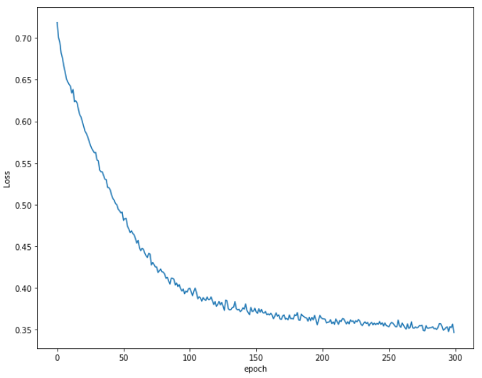
The output shows that initially the loss decreases rapidly. After around the 250th epoch, there is a very little decrease in the loss.

Making Predictions

The last step is to make predictions on the test data. To do so, we simply need to pass the categorical_test_data and numerical_test_data to the model class. The values returned can then be compared with the actual test output values. The following script makes predictions on the test class and prints the cross entropy loss for the test data.

with torch.no_grad():
    y_val = model(categorical_test_data, numerical_test_data)
    loss = loss_function(y_val, test_outputs)
print(f'Loss: {loss:.8f}')

Output:

Loss: 0.36855841

The loss on the test set is 0.3685, which is slightly more than 0.3465 achieved on the training set which shows that our model is slightly overfitting.

It is important to note that since we specified that our output layer will contain 2 neurons, each prediction will contain 2 values. For instance, the first 5 predicted values look like this:

print(y_val[:5])

Output:

tensor([[ 1.2045, -1.3857],
        [ 1.3911, -1.5957],
        [ 1.2781, -1.3598],
        [ 0.6261, -0.5429],
        [ 2.5430, -1.9991]])

The idea behind such predictions is that if the actual output is 0, the value at the index 0 should be higher than the value at index 1, and vice versa. We can retrieve the index of the largest value in the list with the following script:

y_val = np.argmax(y_val, axis=1)

Output:

Let's now again print the first five values for the y_val list:

print(y_val[:5])

Output:

tensor([0, 0, 0, 0, 0])

Since in the list of originally predicted outputs, for the first five records, the the values at zero indexes are greater than the values at first indexes, we can see 0 in the first five rows of the processed outputs.

Finally, we can use the confusion_matrix, accuracy_score, and classification_report classes from the sklearn.metrics module to find the accuracy, precision, and recall values for the test set, along with the confusion matrix.

from sklearn.metrics import classification_report, confusion_matrix, accuracy_score

print(confusion_matrix(test_outputs,y_val))
print(classification_report(test_outputs,y_val))
print(accuracy_score(test_outputs, y_val))

Output:

[[1527   83]
 [ 224  166]]
              precision    recall  f1-score   support

           0       0.87      0.95      0.91      1610
           1       0.67      0.43      0.52       390

   micro avg       0.85      0.85      0.85      2000
   macro avg       0.77      0.69      0.71      2000
weighted avg       0.83      0.85      0.83      2000

0.8465

The output shows that our model achieves an accuracy of 84.65% which is pretty impressive given the fact that we randomly selected all the parameters for our neural network model. I would suggest that you try to change the model parameters i.e. train/test splits, number and size of hidden layers, etc. to see if you can get better results.

Conclusion

PyTorch is a commonly used deep learning library developed by Facebook which can be used for a variety of tasks such as classification, regression, and clustering. This article explains how to use the PyTorch library for the classification of tabular data.