Introduction to Reinforcement Learning with Python

Introduction

Reinforcement Learning is definitely one of the most active and stimulating areas of research in AI.

The interest in this field grew exponentially over the last couple of years, following great (and greatly publicized) advances, such as DeepMind's AlphaGo beating the word champion of GO, and OpenAI AI models beating professional DOTA players.

Thanks to all of these advances, Reinforcement Learning is now being applied in a variety of different fields, from health-care to finance, from chemistry to resource management.

In this article, we will introduce the fundamental concepts and terminology of Reinforcement Learning, and we will apply them in a practical example.

What is Reinforcement Learning?

Reinforcement Learning (RL) is a branch of machine learning concerned with actors, or agents, taking actions is some kind of environment in order to maximize some type of reward that they collect along the way.

This is deliberately a very loose definition, which is why reinforcement learning techniques can be applied to a very wide range of real-world problems.

Imagine someone playing a video game. The player is the agent, and the game is the environment. The rewards the player gets (i.e. beat an enemy, complete a level), or doesn't get (i.e. step into a trap, lose a fight) will teach him how to be a better player.

As you've probably noticed, reinforcement learning doesn't really fit into the categories of supervised/unsupervised/semi-supervised learning.

In supervised learning, for example, each decision taken by the model is independent, and doesn't affect what we see in the future.

In reinforcement learning, instead, we are interested in a long term strategy for our agent, which might include sub-optimal decisions at intermediate steps, and a trade-off between exploration (of unknown paths), and exploitation of what we already know about the environment.

Brief History of Reinforcement Learning

For several decades (since the 1950s!), reinforcement learning followed two separate threads of research, one focusing on trial and error approaches, and one based on optimal control.

Optimal control methods are aimed at designing a controller to minimize a measure of a dynamical system's behavior over time. To achieve this, they mainly used dynamic programming algorithms, which we will see are the foundations of modern reinforcement learning techniques.

Trial-and-error approaches, instead, have deep roots in the psychology of animal learning and neuroscience, and this is where the term reinforcement comes from: actions followed (reinforced) by good or bad outcomes have the tendency to be reselected accordingly.

Arising from the interdisciplinary study of these two fields came a field called Temporal Difference (TD) Learning.

The modern machine learning approaches to RL are mainly based on TD-Learning, which deals with rewards signals and a value function (we'll see more in detail what these are in the following paragraphs).

Terminology

We will now take a look at the main concepts and terminology of Reinforcement Learning.

Agent

A system that is embedded in an environment, and takes actions to change the state of the environment. Examples include mobile robots, software agents, or industrial controllers.

Environment

The external system that the agent can "perceive" and act on.

Environments in RL are defined as Markov Decision Processes (MDPs). A MDP is a tuple:

$$
(S, A, P, R, \gamma)
$$

where:

• S is a finite set of states
• A is a finite set of actions
• P is a state transition probability matrix

• R is a reward function

• γ is a discount factor, γ ∈ [0,1]

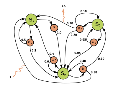
A lot of real-world scenarios can be represented as Markov Decision Processes, from a simple chess board to a much more complex video game.

In a chess environment, the states are all the possible configurations of the board (there are a lot). The actions refer to moving the pieces, surrendering, etc.

The rewards are based on whether we win or lose the game, so that winning actions have higher return than losing ones.

State transition probabilities enforce the game rules. For example, an illegal action (move a rook diagonally) will have zero probability.

Reward Function

The reward function maps states to their rewards. This is the information that the agents use to learn how to navigate the environment.

A lot of research goes into designing a good reward function and overcoming the problem of sparse rewards, when the often sparse nature of rewards in the environment doesn't allow the agent to learn properly from it.

Return G_t is defined as the discounted sum of rewards from time step t.

γ is called the discount factor, and it works by reducing the amount of the rewards as we move into the future.

Discounting rewards allows us to represent uncertainty about the future, but it also helps us model human behavior better, since it has been shown that humans/animals have a preference for immediate rewards.

Value Function

The value function is probably the most important piece of information we can hold about a RL problem.

Formally, the value function is the expected return starting from state s. In practice, the value function tells us how good it is for the agent to be in a certain state. The higher the value of a state, the higher the amount of reward we can expect:

The actual name for this function is state-value function, to distinguish it from another important element in RL: the action-value function.

The action-value function gives us the value, i.e. the expected return, for using action a in a certain state s:

Policy

The policy defines the behavior of our agent in the MDP.

Formally, policies are distributions over actions given states. A policy maps states to the probability of taking each action from that state:

The ultimate goal of RL is to find an optimal (or a good enough) policy for our agent. In the video game example, you can think of the policy as the strategy that the player follows, i.e, the actions the player takes when presented with certain scenarios.

Main Approaches

A lot of different models and algorithms are being applied to RL problems.

Really, a lot.

However, all of them more or less fall into the same two categories: policy-based, and value-based.

Policy-Based Approach

In policy-based approaches to RL, our goal is to learn the best possible policy. Policy models will directly output the best possible move from the current state, or a distribution over the possible actions.

Value-Based Approach

In value-based approaches, we want to find the optimal value function, which is the maximum value function over all policies.

We can then choose which actions to take (i.e. which policy to use) based on the values we get from the model.

Exploration vs Exploitation

The trade-off between exploration and exploitation has been widely studied in the RL literature.

Exploration refers to the act of visiting and collecting information about states in the environment that we have not yet visited, or about which we still don't have much information. The idea is that exploring our MDP might lead us to better decisions in the future.

On the other side, exploitation consists of making the best decision given current knowledge, comfortable in the bubble of the already known.

We will see in the following example how these concepts apply to a real problem.

A Multi-Armed Bandit

We will now look at a practical example of a Reinforcement Learning problem - the multi-armed bandit problem.

The multi-armed bandit is one of the most popular problems in RL:

You are faced repeatedly with a choice among k different options, or actions. After each choice you receive a numerical reward chosen from a stationary probability distribution that depends on the action you selected. Your objective is to maximize the expected total reward over some time period, for example, over 1000 action selections, or time steps.

You can think of it in analogy to a slot machine (a one-armed bandit). Each action selection is like a play of one of the slot machine’s levers, and the rewards are the payoffs for hitting the jackpot.

Solving this problem means that we can come come up with an optimal policy: a strategy that allows us to select the best possible action (the one with the highest expected return) at each time step.

Action-Value Methods

A very simple solution is based on the action value function. Remember that an action value is the mean reward when that action is selected:

We can easily estimate q using the sample average:

If we collect enough observations, our estimate gets close enough to the real function. We can then act greedily at each timestep, i.e. select the action with the highest value, to collect the highest possible rewards.

Don't be too Greedy

Remember when we talked about the trade-off between exploration and exploitation? This is one example of why we should care about it.

As a matter of fact, if we always act greedily as proposed in the previous paragraph, we never try out sub-optimal actions which might actually eventually lead to better results.

To introduce some degree of exploration in our solution, we can use an ε-greedy strategy: we select actions greedily most of the time, but every once in a while, with probability ε, we select a random action, regardless of the action values.

It turns out that this simple exploration method works very well, and it can significantly increase the rewards we get.

One final caveat - to avoid from making our solution too computationally expensive, we compute the average incrementally according to this formula:

Python Solution Walkthrough

import numpy as np

# Number of bandits
k = 3

# Our action values
Q = [0 for _ in range(k)]

# This is to keep track of the number of times we take each action
N = [0 for _ in range(k)]

# Epsilon value for exploration
eps = 0.1

# True probability of winning for each bandit
p_bandits = [0.45, 0.40, 0.80]

def pull(a):
    """Pull arm of bandit with index `i` and return 1 if win, 
    else return 0."""
    if np.random.rand() < p_bandits[a]:
        return 1
    else:
        return 0

while True:
    if np.random.rand() > eps:
        # Take greedy action most of the time
        a = np.argmax(Q)
    else:
        # Take random action with probability eps
        a = np.random.randint(0, k)
    
    # Collect reward
    reward = pull(a)
    
    # Incremental average
    N[a] += 1
    Q[a] += 1/N[a] * (reward - Q[a])

Et voilà! If we run this script for a couple of seconds, we already see that our action values are proportional to the probability of hitting the jackpots for our bandits:

0.4406301434281669, 
0.39131455399060977, 
0.8008844354479673

This means that our greedy policy will correctly favor actions from which we can expect higher rewards.

Conclusion

Reinforcement Learning is a growing field, and there is a lot more to cover. In fact, we still haven't looked at general-purpose algorithms and models (e.g. dynamic programming, Monte Carlo, Temporal Difference).

The most important thing right now is to get familiar with concepts such as value functions, policies, and MDPs. In the Resources section of this article, you'll find some awesome resources to gain a deeper understanding of this kind of material.

Resources

• David Silver class on RL
• Sutton and Barto - Reinforcement Learning: An Introduction