Overview of Classification Methods in Python with Scikit-Learn

Introduction

Are you a Python programmer looking to get into machine learning? An excellent place to start your journey is by getting acquainted with Scikit-Learn.

Doing some classification with Scikit-Learn is a straightforward and simple way to start applying what you've learned, to make machine learning concepts concrete by implementing them with a user-friendly, well-documented, and robust library.

What is Scikit-Learn?

Scikit-Learn is a library for Python that was first developed by David Cournapeau in 2007. It contains a range of useful algorithms that can easily be implemented and tweaked for the purposes of classification and other machine learning tasks.

Scikit-Learn uses SciPy as a foundation, so this base stack of libraries must be installed before Scikit-Learn can be utilized.

Defining our Terms

Before we go any further into our exploration of Scikit-Learn, let's take a minute to define our terms. It is important to have an understanding of the vocabulary that will be used when describing Scikit-Learn's functions.

To begin with, a machine learning system or network takes inputs and outputs. The inputs into the machine learning framework are often referred to as "features" .

Features are essentially the same as variables in a scientific experiment, they are characteristics of the phenomenon under observation that can be quantified or measured in some fashion.

When these features are fed into a machine learning framework the network tries to discern relevant patterns between the features. These patterns are then used to generate the outputs of the framework/network.

The outputs of the framework are often called "labels", as the output features have some label given to them by the network, some assumption about what category the output falls into.

Credit: Siyavula Education

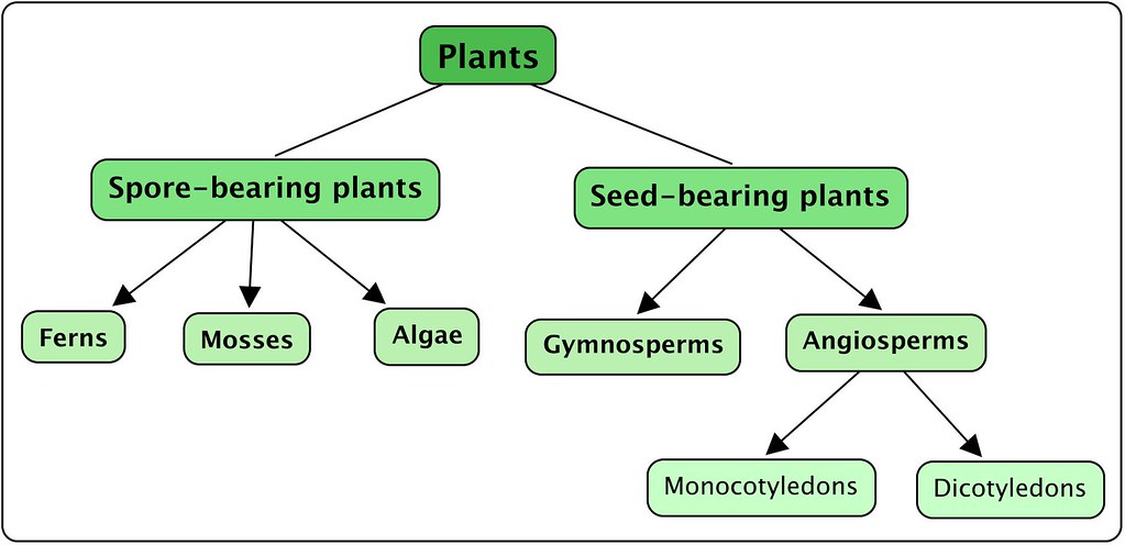
In a machine learning context, classification is a type of supervised learning. Supervised learning means that the data fed to the network is already labeled, with the important features/attributes already separated into distinct categories beforehand.

This means that the network knows which parts of the input are important, and there is also a target or ground truth that the network can check itself against. An example of classification is sorting a bunch of different plants into different categories like ferns or angiosperms. That task could be accomplished with a Decision Tree, a type of classifier in Scikit-Learn.

In contrast, unsupervised learning is where the data fed to the network is unlabeled and the network must try to learn for itself what features are most important. As mentioned, classification is a type of supervised learning, and therefore we won't be covering unsupervised learning methods in this article.

The process of training a model is the process of feeding data into a neural network and letting it learn the patterns of the data. The training process takes in the data and pulls out the features of the dataset. During the training process for a supervised classification task the network is passed both the features and the labels of the training data. However, during testing, the network is only fed features.

The testing process is where the patterns that the network has learned are tested. The features are given to the network, and the network must predict the labels. The data for the network is divided into training and testing sets, two different sets of inputs. You do not test the classifier on the same dataset you train it on, as the model has already learned the patterns of this set of data and it would be extreme bias.

Instead, the dataset is split up into training and testing sets, a set the classifier trains on and a set the classifier has never seen before.

Different Types of Classifiers

Credit: CreativeMagic

Scikit-Learn provides easy access to numerous different classification algorithms. Among these classifiers are:

• K-Nearest Neighbors
• Support Vector Machines
• Decision Tree Classifiers/Random Forests
• Naive Bayes
• Linear Discriminant Analysis
• Logistic Regression

There is a lot of literature on how these various classifiers work, and brief explanations of them can be found at Scikit-Learn's website.

For this reason, we won't delve too deeply into how they work here, but there will be a brief explanation of how the classifier operates.

K-Nearest Neighbors

Credit: Antti Ajanki AnAj

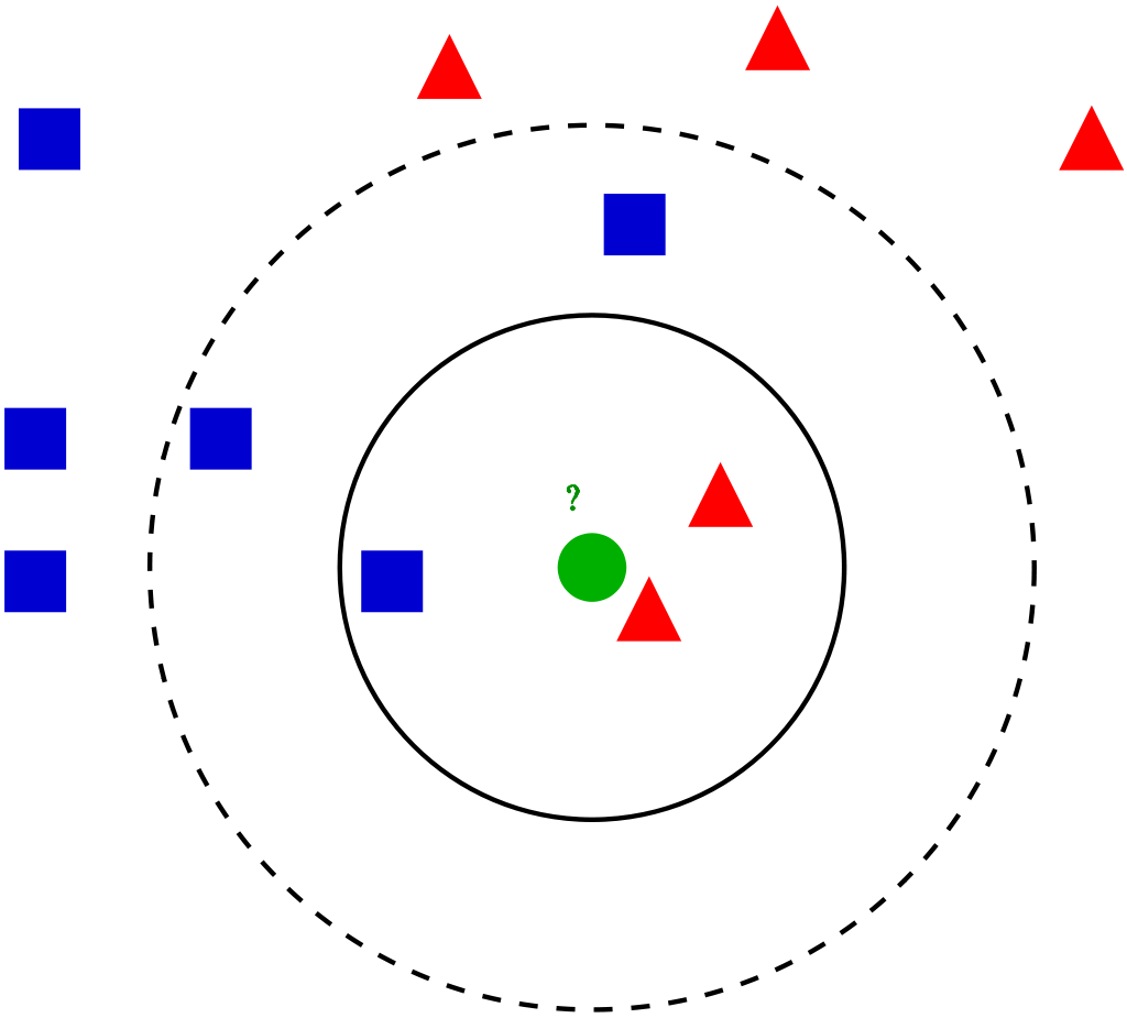
K-Nearest Neighbors operates by checking the distance from some test example to the known values of some training example. The group of data points/class that would give the smallest distance between the training points and the testing point is the class that is selected.

Decision Trees

A Decision Tree Classifier functions by breaking down a dataset into smaller and smaller subsets based on different criteria. Different sorting criteria will be used to divide the dataset, with the number of examples getting smaller with every division.

Once the network has divided the data down to one example, the example will be put into a class that corresponds to a key. When multiple random forest classifiers are linked together they are called Random Forest Classifiers.

Naive Bayes

A Naive Bayes Classifier determines the probability that an example belongs to some class, calculating the probability that an event will occur given that some input event has occurred.

When it does this calculation it is assumed that all the predictors of a class have the same effect on the outcome, that the predictors are independent.

Linear Discriminant Analysis

Linear Discriminant Analysis works by reducing the dimensionality of the dataset, projecting all of the data points onto a line. Then it combines these points into classes based on their distance from a chosen point or centroid.

Linear discriminant analysis, as you may be able to guess, is a linear classification algorithm and best used when the data has a linear relationship.

Support Vector Machines

Credit: Qluong2016

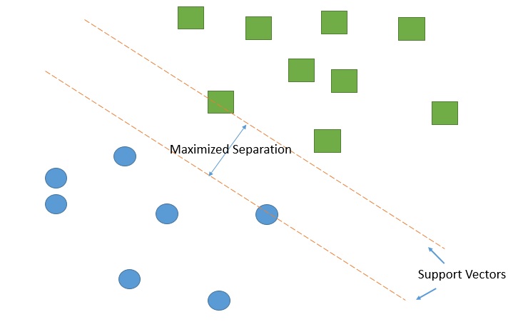
Support Vector Machines work by drawing a line between the different clusters of data points to group them into classes. Points on one side of the line will be one class and points on the other side belong to another class.

The classifier will try to maximize the distance between the line it draws and the points on either side of it, to increase its confidence in which points belong to which class. When the testing points are plotted, the side of the line they fall on is the class they are put in.

Logistic Regression

Logistic Regression outputs predictions about test data points on a binary scale, zero or one. If the value of something is 0.5 or above, it is classified as belonging to class 1, while below 0.5 if is classified as belonging to 0.

Each of the features also has a label of only 0 or 1. Logistic regression is a linear classifier and therefore used when there is some sort of linear relationship between the data.

Examples of Classification Tasks

Classification tasks are any tasks that have you putting examples into two or more classes. Determining if an image is a cat or dog is a classification task, as is determining what the quality of a bottle of wine is based on features like acidity and alcohol content.

Depending on the classification task at hand, you will want to use different classifiers. For instance, a logistic regression model is best suited for binary classification tasks, even though multiple variable logistic regression models exist.

As you gain more experience with classifiers you will develop a better sense for when to use which classifier. However, a common practice is to instantiate multiple classifiers and compare their performance against one another, then select the classifier which performs the best.

Implementing a Classifier

Now that we've discussed the various classifiers that Scikit-Learn provides access to, let's see how to implement a classifier.

The first step in implementing a classifier is to import the classifier you need into Python. Let's look at the import statement for logistic regression:

from sklearn.linear_model import LogisticRegression

Here are the import statements for the other classifiers discussed in this article:

from sklearn.discriminant_analysis import LinearDiscriminantAnalysis
from sklearn.neighbors import KNeighborsClassifier
from sklearn.naive_bayes import GaussianNB
from sklearn.tree import DecisionTreeClassifier
from sklearn.svm import SVC

Scikit-Learn has other classifiers as well, and their respective documentation pages will show how to import them.

After this, the classifier must be instantiated. Instantiation is the process of bringing the classifier into existence within your Python program - to create an instance of the classifier/object.

This is typically done just by making a variable and calling the function associated with the classifier:

logreg_clf = LogisticRegression()

Now the classifier needs to be trained. In order to accomplish this, the classifier must be fit with the training data.

The training features and the training labels are passed into the classifier with the fit command:

logreg_clf.fit(features, labels)

After the classifier model has been trained on the training data, it can make predictions on the testing data.

This is easily done by calling the predict command on the classifier and providing it with the parameters it needs to make predictions about, which are the features in your testing dataset:

logreg_clf.predict(test_features)

These steps: instantiation, fitting/training, and predicting are the basic workflow for classifiers in Scikit-Learn.

However, the handling of classifiers is only one part of doing classifying with Scikit-Learn. The other half of the classification in Scikit-Learn is handling data.

To understand how handling the classifier and handling data come together as a whole classification task, let's take a moment to understand the machine learning pipeline.

The Machine Learning Pipeline

The machine learning pipeline has the following steps: preparing data, creating training/testing sets, instantiating the classifier, training the classifier, making predictions, evaluating performance, tweaking parameters.

The first step to training a classifier on a dataset is to prepare the dataset - to get the data into the correct form for the classifier and handle any anomalies in the data. If there are missing values in the data, outliers in the data, or any other anomalies these data points should be handled, as they can negatively impact the performance of the classifier. This step is referred to as data preprocessing.

Once the data has been preprocessed, the data must be split into training and testing sets. We have previously discussed the rationale for creating training and testing sets, and this can easily be done in Scikit-Learn with a helpful function called train_test_split.

As previously discussed the classifier has to be instantiated and trained on the training data. After this, predictions can be made with the classifier. By comparing the predictions made by the classifier to the actual known values of the labels in your test data, you can get a measurement of how accurate the classifier is.

There are various methods comparing the hypothetical labels to the actual labels and evaluating the classifier. We'll go over these different evaluation metrics later. For now, know that after you've measured the classifier's accuracy, you will probably go back and tweak the parameters of your model until you have hit an accuracy you are satisfied with (as it is unlikely your classifier will meet your expectations on the first run).

Let's look at an example of the machine learning pipeline, going from data handling to evaluation.

Sample Classification Implementation

# Begin by importing all necessary libraries
import pandas as pd
from sklearn.metrics import classification_report
from sklearn.metrics import confusion_matrix
from sklearn.metrics import accuracy_score
from sklearn.neighbors import KNeighborsClassifier
from sklearn.svm import SVC

Because the iris dataset is so common, Scikit-Learn actually already has it, available for loading in with the following command:

sklearn.datasets.load_iris

However, we'll be loading the CSV file here, so that you get a look at how to load and preprocess data. You can download the CSV file here.

Just put the data file in the same directory as your Python file. The Pandas library has an easy way to load in data, read_csv():

data = pd.read_csv('iris.csv')
    
# It is a good idea to check and make sure the data is loaded as expected.
    
print(data.head(5))

Because the dataset has been prepared so well, we don't need to do a lot of preprocessing. One thing we may want to do though is drop the "ID" column, as it is just a representation of the row the example is found on.

As this isn't helpful we could drop it from the dataset using the drop() function:

data.drop('Id', axis=1, inplace=True)

We now need to define the features and labels. We can do this easily with Pandas by slicing the data table and choosing certain rows/columns with iloc():

# Pandas ".iloc" expects row_indexer, column_indexer  
X = data.iloc[:,:-1].values
# Now let's tell the dataframe which column we want for the target/labels.  
y = data['Species']

The slicing notation above selects every row and every column except the last column (which is our label, the species).

Alternatively, you could select certain features of the dataset you were interested in by using the bracket notation and passing in column headers:

# Alternate way of selecting columns:
X = data.iloc['SepalLengthCm', 'SepalWidthCm', 'PetalLengthCm']

Now that we have the features and labels we want, we can split the data into training and testing sets using sklearn's handy feature train_test_split():

# Test size specifies how much of the data you want to set aside for the testing set. 
# Random_state parameter is just a random seed we can use.
# You can use it if you'd like to reproduce these specific results.
X_train, X_test, y_train, y_test = train_test_split(X, y, test_size=0.20, random_state=27)

You may want to print the results to be sure your data is being parsed as you expect:

print(X_train)  
print(y_train)

Now we can instantiate the models. Let's try using two classifiers, a Support Vector Classifier and a K-Nearest Neighbors Classifier:

SVC_model = svm.SVC()
# KNN model requires you to specify n_neighbors,
# the number of points the classifier will look at to determine what class a new point belongs to
KNN_model = KNeighborsClassifier(n_neighbors=5)

Now let's fit the classifiers:

SVC_model.fit(X_train, y_train)
KNN_model.fit(X_train, y_train)

The call has trained the model, so now we can predict and store the prediction in a variable:

SVC_prediction = SVC_model.predict(X_test)
KNN_prediction = KNN_model.predict(X_test)

We should now evaluate how the classifier performed. There are multiple methods of evaluating a classifier's performance, and you can read more about their different methods below.

In Scikit-Learn you just pass in the predictions against the ground truth labels which were stored in your test labels:

# Accuracy score is the simplest way to evaluate
print(accuracy_score(SVC_prediction, y_test))
print(accuracy_score(KNN_prediction, y_test))
# But Confusion Matrix and Classification Report give more details about performance
print(confusion_matrix(SVC_prediction, y_test))
print(classification_report(KNN_prediction, y_test))

For reference, here's the output we got on the metrics:

SVC accuracy: 0.9333333333333333
KNN accuracy: 0.9666666666666667

At first glance, it seems KNN performed better. Here's the confusion matrix for SVC:

[[ 7  0  0]
 [ 0 10  1]
 [ 0  1 11]]

This can be a bit hard to interpret, but the number of correct predictions for each class run on the diagonal from top-left to bottom-right. Check below for more info on this.

Finally, here's the output for the classification report for KNN:

precision    recall  f1-score   support
    
Iris-setosa       1.00      1.00      1.00         7
Iris-versicolor       0.91      0.91      0.91        11
Iris-virginica       0.92      0.92      0.92        12
    
micro avg       0.93      0.93      0.93        30
macro avg       0.94      0.94      0.94        30
weighted avg       0.93      0.93      0.93        30

Evaluating the Classifier

When it comes to the evaluation of your classifier, there are several different ways you can measure its performance.

Classification Accuracy

Classification Accuracy is the simplest out of all the methods of evaluating the accuracy, and the most commonly used. Classification accuracy is simply the number of correct predictions divided by all predictions or a ratio of correct predictions to total predictions.

While it can give you a quick idea of how your classifier is performing, it is best used when the number of observations/examples in each class is roughly equivalent. Because this doesn't happen very often, you're probably better off using another metric.

Logarithmic Loss

Logarithmic Loss, or LogLoss, essentially evaluates how confident the classifier is about its predictions. LogLoss returns probabilities for membership of an example in a given class, summing them together to give a representation of the classifier's general confidence.

The value for predictions runs from 1 to 0, with 1 being completely confident and 0 being no confidence. The loss, or overall lack of confidence, is returned as a negative number with 0 representing a perfect classifier, so smaller values are better.

Area Under ROC Curve (AUC)

This is a metric used only for binary classification problems. The area under the curve represents the model's ability to properly discriminate between negative and positive examples, between one class or another.

A 1.0, all of the area falling under the curve, represents a perfect classifier. This means that an AUC of 0.5 is basically as good as randomly guessing. The ROC curve is calculated with regards to sensitivity (true positive rate/recall) and specificity (true negative rate). You can read more about these calculations at this ROC curve article.

Confusion Matrix

A confusion matrix is a table or chart, representing the accuracy of a model with regards to two or more classes. The predictions of the model will be on the X-axis while the outcomes/accuracy are located on the y-axis.

The cells are filled with the number of predictions the model makes. Correct predictions can be found on a diagonal line moving from the top left to the bottom right. You can read more about interpreting a confusion matrix here.

Classification Report

The classification report is a Scikit-Learn built in metric created especially for classification problems. Using the classification report can give you a quick intuition of how your model is performing. Recall pits the number of examples your model labeled as Class A (some given class) against the total number of examples of Class A, and this is represented in the report.

The report also returns prediction and f1-score. Precision is the percentage of examples your model labeled as Class A which actually belonged to Class A (true positives against false positives), and f1-score is an average of precision and recall.

Conclusion

To take your understanding of Scikit-Learn farther, it would be a good idea to learn more about the different classification algorithms available. Once you have an understanding of these algorithms, read more about how to evaluate classifiers.

Many of the nuances of classification only come with time and practice, but if you follow the steps in this guide you'll be well on your way to becoming an expert in classification tasks with Scikit-Learn.