Python for NLP: Creating TF-IDF Model from Scratch

This is the 14th article in my series of articles on Python for NLP. In my previous article, I explained how to convert sentences into numeric vectors using the bag of words approach. To get a better understanding of the bag of words approach, we implemented the technique in Python.

In this article, we will build upon the concept that we learn in the last article and will implement the TF-IDF scheme from scratch in Python. The term TF stands for "term frequency" while the term IDF stands for the "inverse document frequency".

Problem with Bag of Words Model

Before we actually see the TF-IDF model, let us first discuss a few problems associated with the bag of words model.

In the last article, we had the following three example sentences:

• "I like to play football"
• "Did you go outside to play tennis"
• "John and I play tennis"

The resulting bag of words model looked like this:

	Play	Tennis	To	I	Football	Did	You	go
Sentence 1	1	0	1	1	1	0	0	0
Sentence 2	1	1	1	0	0	1	1	1
Sentence 3	1	1	0	1	0	0	0	0

One of the main problems associated with the bag of words model is that it assigns equal value to the words, irrespective of their importance. For instance, the word "play" appears in all the three sentences, therefore this word is very common, on the other hand, the word "football" only appears in one sentence. The words that are rare have more classifying power compared to the words that are common.

The idea behind the TF-IDF approach is that the words that are more common in one sentence and less common in other sentences should be given high weights.

Theory Behind TF-IDF

Before implementing the TF-IDF scheme in Python, let's first study the theory. We will use the same three sentences as our example as we used in the bag of words model.

• "I like to play football"
• "Did you go outside to play tennis"
• "John and I play tennis"

Step 1: Tokenization

Like the bag of words, the first step to implement the TF-IDF model is tokenization.

Sentence 1	Sentence 2	Sentence 3
I	Did	John
like	you	and
to	go	I
play	outside	play
football	to	tennis
	play
	tennis

Step 2: Find TF-IDF Values

Once you have tokenized the sentences, the next step is to find the TF-IDF value for each word in the sentence.

As discussed earlier, the TF value refers to term frequency and can be calculated as follows:

TF = (Frequency of the word in the sentence) / (Total number of words in the sentence)

For instance, look at the word "play" in the first sentence. Its term frequency will be 0.20 since the word "play" occurs only once in the sentence and the total number of words in the sentence are 5, hence, 1/5 = 0.20.

IDF refers to inverse document frequency and can be calculated as follows:

IDF: (Total number of sentences (documents))/(Number of sentences (documents) containing the word)

It is important to mention that the IDF value for a word remains the same throughout all the documents as it depends upon the total number of documents. On the other hand, TF values of a word differ from document to document.

Let's find the IDF frequency of the word "play". Since we have three documents and the word "play" occurs in all three of them, therefore the IDF value of the word "play" is 3/3 = 1.

Finally, the TF-IDF values are calculated by multiplying TF values with their corresponding IDF values.

To find the TF-IDF value, we first need to create a dictionary of word frequencies as shown below:

Word	Frequency
I	2
like	1
to	2
play	3
football	1
Did	1
you	1
go	1
outside	1
tennis	2
John	1
and	1

Next, let's sort the dictionary in the descending order of the frequency as shown in the following table.

Word	Frequency
play	3
tennis	2
to	2
I	2
football	1
Did	1
you	1
go	1
outside	1
like	1
John	1
and	1

Finally, we will filter the 8 most frequently occurring words.

As I said earlier, since IDF values are calculated using the whole corpus, we can calculate the IDF value for each word now. The following table contains IDF values for each table.

Word	Frequency	IDF
play	3	3/3 = 1
tennis	2	3/2 = 1.5
to	2	3/2 = 1.5
I	2	3/2 = 1.5
football	1	3/1 = 3
Did	1	3/1 = 3
you	1	3/1 = 3
go	1	3/1 = 3

You can clearly see that the words that are rare have higher IDF values compared to the words that are more common.

Let's now find the TF-IDF values for all the words in each sentence.

Word	Sentence 1	Sentence 2	Sentence 3
play	0.20 x 1 = 0.20	0.14 x 1 = 0.14	0.20 x 1 = 0.20
tennis	0 x 1.5 = 0	0.14 x 1.5 = 0.21	0.20 x 1.5 = 0.30
to	0.20 x 1.5 = 0.30	0.14 x 1.5 = 0.21	0 x 1.5 = 0
I	0.20 x 1.5 = 0.30	0 x 1.5 = 0	0.20 x 1.5 = 0.30
football	0.20 x 3 = 0.6	0 x 3 = 0	0 x 3 = 0
did	0 x 3 = 0	0.14 x 3 = 0.42	0 x 3 = 0
you	0 x3 = 0	0.14 x 3 = 0.42	0 x 3 = 0
go	0x 3 = 0	0.14 x 3 = 0.42	0 x 3 = 0

The values in the columns for sentence 1, 2, and 3 are corresponding TF-IDF vectors for each word in the respective sentences.

Note the use of the log function with TF-IDF.

It is important to mention that to mitigate the effect of very rare and very common words on the corpus, the log of the IDF value can be calculated before multiplying it with the TF-IDF value. In such case the formula of IDF becomes:

IDF: log((Total number of sentences (documents))/(Number of sentences (documents) containing the word))

However, since we had only three sentences in our corpus, for the sake of simplicity we did not use log. In the implementation section, we will use the log function to calculate the final TF-IDF value.

TF-IDF Model from Scratch in Python

As explained in the theory section, the steps to create a sorted dictionary of word frequency is similar between the bag of words and the TF-IDF model. To understand how we create a sorted dictionary of word frequencies, please refer to my last article. Here, I will just write the code. The TF-IDF model will be built upon this code.

# -*- coding: utf-8 -*-
"""
Created on Sat Jul 6 14:21:00 2019

@author: usman
"""

import nltk
import numpy as np
import random
import string

import bs4 as bs
import urllib.request
import re

raw_html = urllib.request.urlopen('https://en.wikipedia.org/wiki/Natural_language_processing')
raw_html = raw_html.read()

article_html = bs.BeautifulSoup(raw_html, 'lxml')

article_paragraphs = article_html.find_all('p')

article_text = ''

for para in article_paragraphs:
    article_text += para.text

corpus = nltk.sent_tokenize(article_text)

for i in range(len(corpus )):
    corpus [i] = corpus [i].lower()
    corpus [i] = re.sub(r'\W',' ',corpus [i])
    corpus [i] = re.sub(r'\s+',' ',corpus [i])

wordfreq = {}
for sentence in corpus:
    tokens = nltk.word_tokenize(sentence)
    for token in tokens:
        if token not in wordfreq.keys():
            wordfreq[token] = 1
        else:
            wordfreq[token] += 1

import heapq
most_freq = heapq.nlargest(200, wordfreq, key=wordfreq.get)

In the above script, we first scrape the Wikipedia article on Natural Language Processing. We then preprocess it to remove all the special characters and multiple empty spaces. Finally, we create a dictionary of word frequencies and then filter the top 200 most frequently occurring words.

The next step is to find the IDF values for the most frequently occurring words in the corpus. The following script does that:

word_idf_values = {}
for token in most_freq:
    doc_containing_word = 0
    for document in corpus:
        if token in nltk.word_tokenize(document):
            doc_containing_word += 1
    word_idf_values[token] = np.log(len(corpus)/(1 + doc_containing_word))

In the script above, we create an empty dictionary word_idf_values. This dictionary will store most frequently occurring words as keys and their corresponding IDF values as dictionary values. Next, we iterate through the list of most frequently occurring words. During each iteration, we create a variable doc_containing_word. This variable will store the number of documents in which the word appears. Next, we iterate through all the sentences in our corpus. The sentence is tokenized and then we check if the word exists in the sentence or not, if the word exists, we increment the doc_containing_word variable. Finally, to calculate the IDF value we divide the total number of sentences by the total number of documents containing the word.

The next step is to create the TF dictionary for each word. In the TF dictionary, the key will be the most frequently occuring words, while values will be 49 dimensional vectors since our document has 49 sentences. Each value in the vector will belong to the TF value of the word for the corresponding sentence. Look at the following script:

word_tf_values = {}
for token in most_freq:
    sent_tf_vector = []
    for document in corpus:
        doc_freq = 0
        for word in nltk.word_tokenize(document):
            if token == word:
                  doc_freq += 1
        word_tf = doc_freq/len(nltk.word_tokenize(document))
        sent_tf_vector.append(word_tf)
    word_tf_values[token] = sent_tf_vector

In the above script, we create a dictionary that contains the word as the key and a list of 49 items as a value since we have 49 sentences in our corpus. Each item in the list stores the TF value of the word for the corresponding sentence. In the script above word_tf_values is our dictionary. For each word, we create a list sent_tf_vector.

We then iterate through each sentence in the corpus and tokenize the sentence. The word from the outer loop is matched with each word in the sentence. If a match is found the doc_freq variable is incremented by 1. Once all the words in the sentence are iterated, the doc_freq is divided by the total length of the sentence to find the TF value of the word for that sentence. This process repeats for all the words in the most frequently occurring word list. The final word_tf_values dictionary will contain 200 words as keys. For each word, there will be a list of 49 items as the value.

If you look at the word_tf_values dictionary, it looks like this:

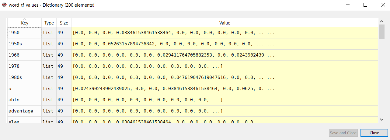
You can see that the word is the key whereas a list of 49 items is the value for each key.

Now we have IDF values of all the words, along with TF values of every word across the sentences. The next step is to simply multiply IDF values with TF values.

tfidf_values = []
for token in word_tf_values.keys():
    tfidf_sentences = []
    for tf_sentence in word_tf_values[token]:
        tf_idf_score = tf_sentence * word_idf_values[token]
        tfidf_sentences.append(tf_idf_score)
    tfidf_values.append(tfidf_sentences)

In the above script, we create a list called tfidf_values. We then iterated through all the keys in the word_tf_values dictionary. These keys are basically the most frequently occurring words. Using these words, we retrieve the 49-dimensional list that contains the TF values for the word corresponding to each sentence. Next, the TF value is multiplied by the IDF value of the word and stored in the tf_idf_score variable. The variable is then appended to the tf_idf_sentences list. Finally, the tf_idf_sentences list is appended to the tfidf_values list.

Now at this point in time, the tfidf_values is a list of lists. Where each item is a 49-dimensional list that contains TF IDF values of a particular word for all the sentences. We need to convert the two-dimensional list to a numpy array. Look at the following script:

tf_idf_model = np.asarray(tfidf_values)

Now, our numpy array looks like this:

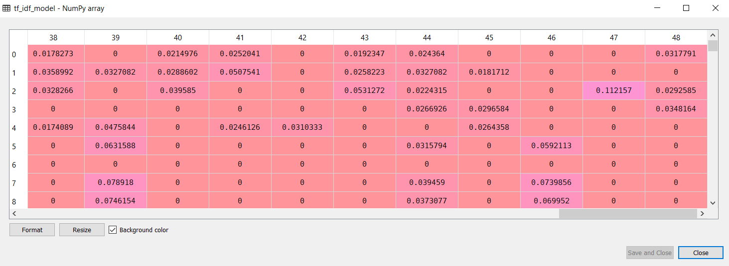
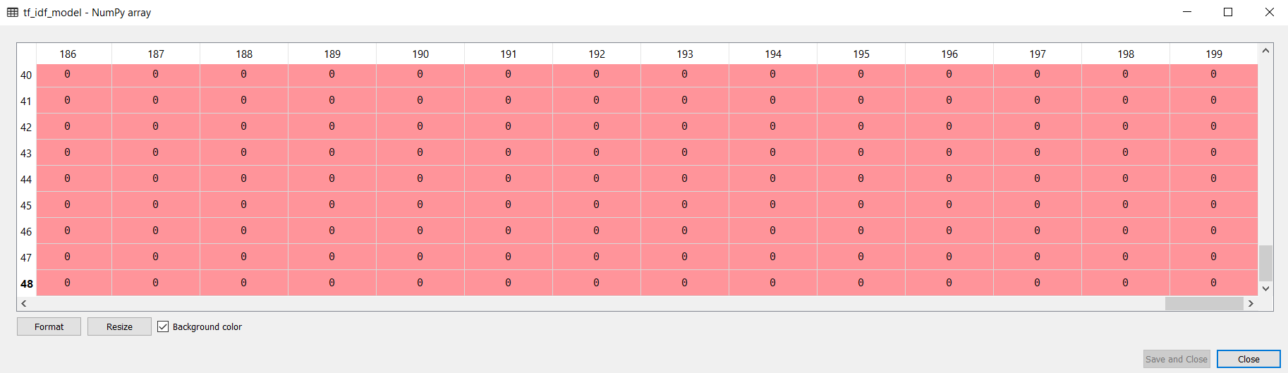
However, there is still one problem with this TF-IDF model. The array dimension is 200 x 49, which means that each column represents the TF-IDF vector for the corresponding sentence. We want rows to represent the TF-IDF vectors. We can do so by simply transposing our numpy array as follows:

tf_idf_model = np.transpose(tf_idf_model)

Now we have 49 x 200-dimensional numpy array where rows correspond to TF-IDF vectors, as shown below:

Conclusion

TF-IDF model is one of the most widely used models for text to numeric conversion. In this article, we briefly reviewed the theory behind the TF-IDF model. Finally, we implemented a TF-IDF model from scratch in Python. In the next article, we will see how to implement the N-Gram model from scratch in Python.