Seaborn Line Plot - Tutorial and Examples

Introduction

Seaborn is one of the most widely used data visualization libraries in Python, as an extension to Matplotlib. It offers a simple, intuitive, yet highly customizable API for data visualization.

In this tutorial, we'll take a look at how to plot a Line Plot in Seaborn - one of the most basic types of plots.

Line Plots display numerical values on one axis, and categorical values on the other.

They can typically be used in much the same way Bar Plots can be used, though, they're more commonly used to keep track of changes over time.

Plot a Line Plot with Seaborn

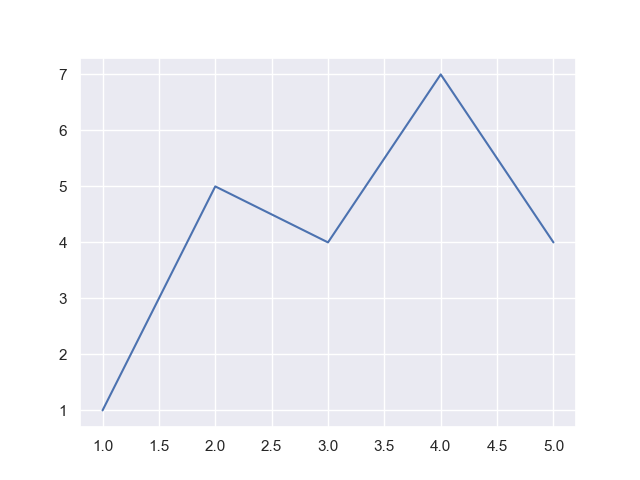
Let's start out with the most basic form of populating data for a Line Plot, by providing a couple of lists for the X-axis and Y-axis to the lineplot() function:

import matplotlib.pyplot as plt
import seaborn as sns

sns.set_theme(style="darkgrid")

x = [1, 2, 3, 4, 5]
y = [1, 5, 4, 7, 4]

sns.lineplot(x, y)
plt.show()

Here, we have two lists of values, x and y. The x list acts as our categorical variable list, while the y list acts as the numerical variable list.

This code results in:

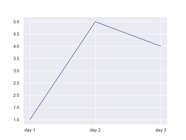
To that end, we can use other data types, such as strings for the categorical axis:

import matplotlib.pyplot as plt
import seaborn as sns

sns.set_theme(style="darkgrid")

x = ['day 1', 'day 2', 'day 3']
y = [1, 5, 4]

sns.lineplot(x, y)
plt.show()

And this would result in:

Note: If you're using integers as your categorical list, such as [1, 2, 3, 4, 5], but then proceed to go to 100, all values between 5..100 will be null:

import seaborn as sns

sns.set_theme(style="darkgrid")

x = [1, 2, 3, 4, 5, 10, 100]
y = [1, 5, 4, 7, 4, 5, 6]

sns.lineplot(x, y)
plt.show()

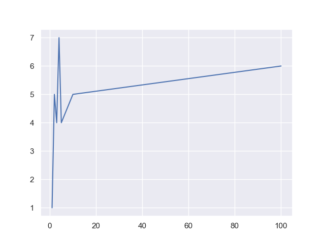
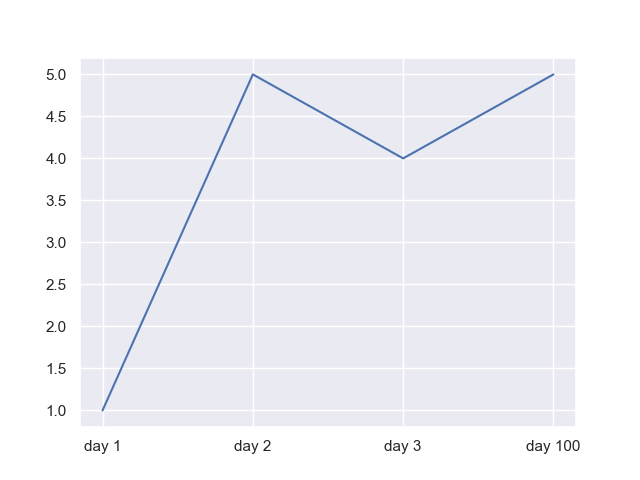
This is because a dataset might simply be missing numerical values on the X-axis. In that case, Seaborn simply lets us assume that those values are missing and plots away. However, when you work with strings, this won't be the case:

import matplotlib.pyplot as plt
import seaborn as sns

sns.set_theme(style="darkgrid")

x = ['day 1', 'day 2', 'day 3', 'day 100']
y = [1, 5, 4, 5]

sns.lineplot(x, y)
plt.show()

However, more typically, we don't work with simple, hand-made lists like this. We work with data imported from larger datasets or pulled directly from databases. Let's import a dataset and work with it instead.

Import Data

Let's use the Hotel Bookings dataset and use the data from there:

import pandas as pd
df = pd.read_csv('hotel_bookings.csv')
print(df.head())

Let's take a look at the columns of this dataset:

          hotel  is_canceled reservation_status  ... arrival_date_month  stays_in_week_nights
0  Resort Hotel            0          Check-Out  ...               July                     0
1  Resort Hotel            0          Check-Out  ...               July                     0
2  Resort Hotel            0          Check-Out  ...               July                     1
3  Resort Hotel            0          Check-Out  ...               July                     1
4  Resort Hotel            0          Check-Out  ...               July                     2

This is a truncated view, since there are a lot of columns in this dataset. For example, let's explore this dataset, by using the arrival_date_month as our categorical X-axis, while we use the stays_in_week_nights as our numerical Y-axis:

import matplotlib.pyplot as plt
import seaborn as sns
import pandas as pd

sns.set_theme(style="darkgrid")

df = pd.read_csv('hotel_bookings.csv')

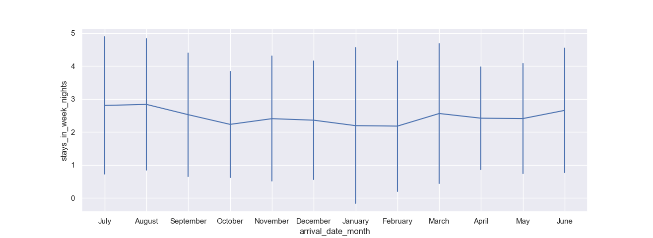
sns.lineplot(x = "arrival_date_month", y = "stays_in_week_nights", data = df)
plt.show()

We've used Pandas to read in the CSV data and pack it into a DataFrame. Then, we can assign the x and y arguments of the lineplot() function as the names of the columns in that dataframe. Of course, we'll have to specify which dataset we're working with by assigning the dataframe to the data argument.

Now, this results in:

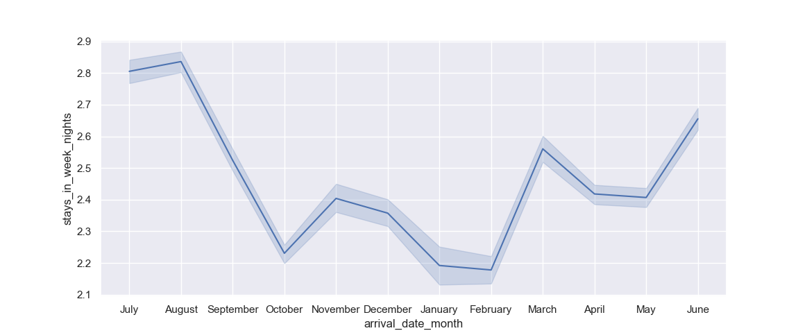
We can clearly see that weeknight stays tend to be longer during the months of June, July and August (summer vacation), while they're the lowest in January and February, right after the chain of holidays leading up to New Year.

Additionally, you can see the confidence interval as the area around the line itself, which is the estimated central tendency of our data. Since we have multiple y values for each x value (many people stayed in each month), Seaborn calculates the central tendency of these records and plots that line, as well as a confidence interval for that tendency.

In general, people stay ~2.8 days on weeknights, in July, but the confidence interval spans from 2.78-2.84.

Plotting Wide-Form Data

Now, let's take a look at how we can plot wide-form data, rather than tidy-form as we've been doing so far. We'll want to visualize the stays_in_week_nights variable over the months, but we'll also want to take the year of that arrival into consideration. This will result in a Line Plot for each year, over the months, on a single figure.

Since the dataset isn't well-suited for this by default, we'll have to do some data preprocessing on it.

import matplotlib.pyplot as plt
import seaborn as sns
import pandas as pd

df = pd.read_csv('hotel_bookings.csv')

# Truncate
df = df[['arrival_date_year', 'arrival_date_month', 'stays_in_week_nights']]
# Save the order of the arrival months
order = df['arrival_date_month']
# Pivot the table to turn it into wide-form
df_wide = df.pivot_table(index='arrival_date_month', columns='arrival_date_year', values='stays_in_week_nights')
# Reindex the DataFrame with the `order` variable to keep the same order of months as before
df_wide = df_wide.reindex(order, axis=0)

print(df_wide)

Here, we've firstly truncated the dataset to a few relevant columns. Then, we've saved the order of arrival date months so we can preserve it for later. You can put in any order here, though.

Then, to turn the narrow-form data into a wide-form, we've pivoted the table around the arrival_date_month feature, turning arrival_date_year into columns, and stays_in_week_nights into values. Finally, we've used reindex() to enforce the same order of arrival months as we had before.

Let's take a look at how our dataset looks like now:

arrival_date_year       2015      2016      2017
arrival_date_month
July                2.789625  2.836177  2.787502
July                2.789625  2.836177  2.787502
July                2.789625  2.836177  2.787502
July                2.789625  2.836177  2.787502
July                2.789625  2.836177  2.787502
...                      ...       ...       ...
August              2.654153  2.859964  2.956142
August              2.654153  2.859964  2.956142
August              2.654153  2.859964  2.956142
August              2.654153  2.859964  2.956142
August              2.654153  2.859964  2.956142

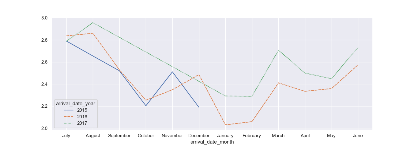
Great! Our dataset is now correctly formatted for wide-form visualization, with the central tendency of the stays_in_week_nights calculated. Now that we're working with a wide-form dataset, all we have to do to plot it is:

sns.lineplot(data=df_wide)
plt.show()

The lineplot() function can natively recognize wide-form datasets and plots them accordingly. This results in:

Customizing Line Plots with Seaborn

Now that we've explored how to plot manually inserted data, how to plot simple dataset features, as well as manipulate a dataset to conform to a different type of visualization - let's take a look at how we can customize our line plots to provide more easy-to-digest information.

Plotting Line Plot with Hues

Hues can be used to segregate a dataset into multiple individual line plots, based on a feature you'd like them to be grouped (hued) by. For example, we can visualize the central tendency of the stays_in_week_nights feature, over the months, but take the arrival_date_year into consideration as well and group individual line plots based on that feature.

This is exactly what we've done in the previous example - manually. We've converted the dataset into a wide-form dataframe and plotted it. However, we could've grouped the years into hues as well, which would net us the exact same result:

import matplotlib.pyplot as plt
import seaborn as sns
import pandas as pd

df = pd.read_csv('hotel_bookings.csv')

sns.lineplot(x = "arrival_date_month", y = "stays_in_week_nights", hue='arrival_date_year', data = df)
plt.show()

By setting the arrival_date_year feature as the hue argument, we've told Seaborn to segregate each X-Y mapping by the arrival_date_year feature, so we'll end up with three different line plots:

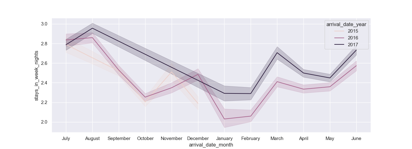
This time around, we've also got confidence intervals marked around our central tendencies.

Customize Line Plot Confidence Interval with Seaborn

You can fiddle around, enable/disable and change the type of confidence intervals easily using a couple of arguments. The ci argument can be used to specify the size of the interval, and can be set to an integer, 'sd' (standard deviation) or None if you want to turn it off.

The err_style can be used to specify the style of the confidence intervals - band or bars. We've seen how bands work so far, so let's try out a confidence interval that uses bars instead:

import matplotlib.pyplot as plt
import seaborn as sns
import pandas as pd

df = pd.read_csv('hotel_bookings.csv')

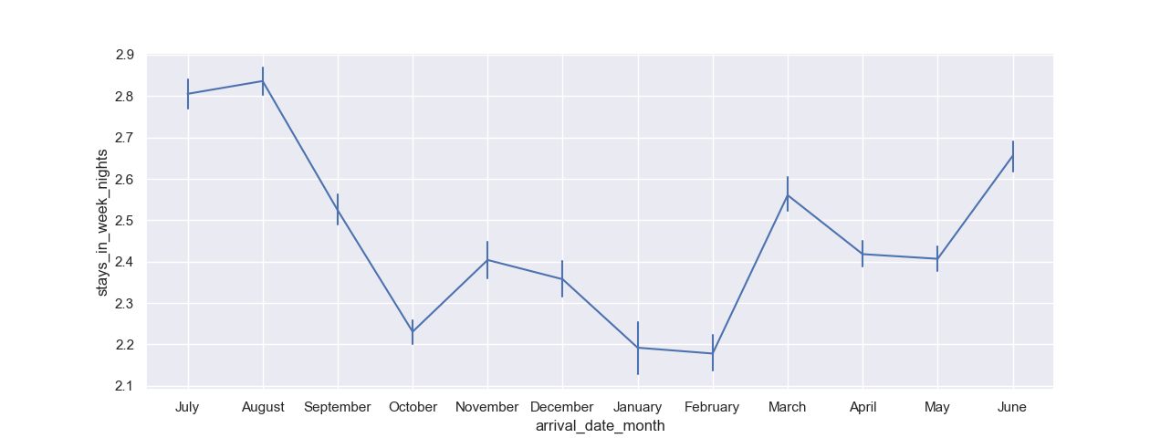
sns.lineplot(x = "arrival_date_month", y = "stays_in_week_nights", err_style='bars', data = df)
plt.show()

This results in:

And let's change the confidence interval, which is by default set to 95, to display standard deviation instead:

import matplotlib.pyplot as plt
import seaborn as sns
import pandas as pd

df = pd.read_csv('hotel_bookings.csv')

sns.lineplot(x = "arrival_date_month", y = "stays_in_week_nights", err_style='bars', ci='sd', data = df)
plt.show()

Conclusion

In this tutorial, we've gone over several ways to plot a Line Plot in Seaborn. We've taken a look at how to plot simple plots, with numerical and categorical X-axes, after which we've imported a dataset and visualized it.

We've explored how to manipulate datasets and change their form to visualize multiple features, as well as how to customize Line Plots.

If you're interested in Data Visualization and don't know where to start, make sure to check out our bundle of books on Data Visualization in Python:

Data Visualization in Python with Matplotlib and Pandas is a book designed to take absolute beginners to Pandas and Matplotlib, with basic Python knowledge, and allow them to build a strong foundation for advanced work with these libraries - from simple plots to animated 3D plots with interactive buttons.

It serves as an in-depth guide that'll teach you everything you need to know about Pandas and Matplotlib, including how to construct plot types that aren't built into the library itself.

Data Visualization in Python, a book for beginner to intermediate Python developers, guides you through simple data manipulation with Pandas, covers core plotting libraries like Matplotlib and Seaborn, and shows you how to take advantage of declarative and experimental libraries like Altair. More specifically, over the span of 11 chapters this book covers 9 Python libraries: Pandas, Matplotlib, Seaborn, Bokeh, Altair, Plotly, GGPlot, GeoPandas, and VisPy.

It serves as a unique, practical guide to Data Visualization, in a plethora of tools you might use in your career.