Sorting Algorithms in Java

Introduction

Sorting data means arranging it in a certain order, often in an array-like data structure. You can use various ordering criteria, common ones being sorting numbers from least to greatest or vice-versa, or sorting strings lexicographically. You can even define your own criteria, and we'll go into practical ways of doing that by the end of this article.

If you're interested in how sorting works, we'll cover various algorithms, from inefficient but intuitive solutions, to efficient algorithms which are actually implemented in Java and other languages.

There are various sorting algorithms, and they're not all equally efficient. We'll be analyzing their time complexity in order to compare them and see which ones perform the best.

The list of algorithms you'll learn here is by no means exhaustive, but we have compiled some of the most common and most efficient ones to help you get started,

Note: This article will not be dealing with concurrent sorting, since it's meant for beginners.

Bubble Sort

Explanation

Bubble sort works by swapping adjacent elements if they're not in the desired order. This process repeats from the beginning of the array until all elements are in order.

We know that all elements are in order when we manage to do the whole iteration without swapping at all - then all elements we compared were in the desired order with their adjacent elements, and by extension, the whole array.

Here are the steps for sorting an array of numbers from least to greatest:

• 4 2 1 5 3: The first two elements are in the wrong order, so we swap them.

• 2 4 1 5 3: The second two elements are in the wrong order too, so we swap.

• 2 1 4 5 3: These two are in the right order, 4 < 5, so we leave them alone.

• 2 1 4 5 3: Another swap.

• 2 1 4 3 5: Here's the resulting array after one iteration.

Because at least one swap occurred during the first pass (there were actually three), we need to go through the whole array again and repeat the same process.

By repeating this process, until no more swaps are made, we'll have a sorted array.

The reason this algorithm is called Bubble Sort is because the numbers kind of "bubble up" to the "surface." If you go through our example again, following a particular number (4 is a great example), you'll see it slowly moving to the right during the process.

All numbers move to their respective places bit by bit, left to right, like bubbles slowly rising from a body of water.

If you'd like to read a detailed, dedicated article for Bubble Sort, we've got you covered!

Implementation

We're going to implement Bubble Sort in a similar way we've laid it out in words. Our function enters a while loop in which it goes through the entire array swapping as needed.

We assume the array is sorted, but if we're proven wrong while sorting (if a swap happens), we go through another iteration. The while-loop then keeps going until we manage to pass through the entire array without swapping:

public static void bubbleSort(int[] a) {
    boolean sorted = false;
    int temp;
    while(!sorted) {
        sorted = true;
        for (int i = 0; i < array.length - 1; i++) {
            if (a[i] > a[i+1]) {
                temp = a[i];
                a[i] = a[i+1];
                a[i+1] = temp;
                sorted = false;
            }
        }
    }
}

When using this algorithm we have to be careful how we state our swap condition.

For example, if I had used a[i] >= a[i+1] it could have ended up with an infinite loop, because for equal elements this relation would always be true, and hence always swap them.

Time Complexity

To figure out the time complexity of Bubble Sort, we need to look at the worst possible scenario. What's the maximum number of times we need to pass through the whole array before we've sorted it? Consider the following example:

5 4 3 2 1

In the first iteration, 5 will "bubble up to the surface," but the rest of the elements will stay in descending order. We would have to do one iteration for each element except 1, and then another iteration to check that everything is in order, so a total of 5 iterations.

Expand this to any array of n elements, and that means you need to do n iterations. Looking at the code, that would mean that our while loop can run the maximum of n times.

Each of those n times we're iterating through the whole array (for-loop in the code), meaning the worst case time complexity would be O(n^2).

Note: The time complexity would always be O(n^2) if it weren't for the sorted boolean check, which terminates the algorithm if there aren't any swaps within the inner loop - which means that the array is sorted.

Insertion Sort

Explanation

The idea behind Insertion Sort is dividing the array into the sorted and unsorted subarrays.

The sorted part is of length 1 at the beginning and is corresponding to the first (left-most) element in the array. We iterate through the array and during each iteration, we expand the sorted portion of the array by one element.

Upon expanding, we place the new element into its proper place within the sorted subarray. We do this by shifting all of the elements to the right until we encounter the first element we don't have to shift.

For example, if in the following array, the part in bold is sorted in an ascending order, the following happens:

• 3 5 7 8 4 2 1 9 6: We take 4 and remember that that's what we need to insert. Since 8 > 4, we shift.

• 3 5 7 x 8 2 1 9 6: Where the value of x is not of crucial importance, since it will be overwritten immediately (either by 4 if it's its appropriate place or by 7 if we shift). Since 7 > 4, we shift.

• 3 5 x 7 8 2 1 9 6

• 3 x 5 7 8 2 1 9 6

• 3 4 5 7 8 2 1 9 6

After this process, the sorted portion was expanded by one element, we now have five rather than four elements. Each iteration does this and by the end we'll have the whole array sorted.

If you'd like to read a detailed, dedicated article for Insertion Sort, we've got you covered!

Implementation

public static void insertionSort(int[] array) {
    for (int i = 1; i < array.length; i++) {
        int current = array[i];
        int j = i - 1;
        while(j >= 0 && current < array[j]) {
            array[j+1] = array[j];
            j--;
        }
        // at this point we've exited, so j is either -1
        // or it's at the first element where current >= a[j]
        array[j+1] = current;
    }
}

Time Complexity

Again, we have to look at the worst case scenario for our algorithm, and it will again be the example where the whole array is descending.

This is because in each iteration, we'll have to move the whole sorted list by one, which is O(n). We have to do this for each element in every array, which means it's going to be bounded by O(n^2).

Selection Sort

Explanation

Selection Sort also divides the array into a sorted and unsorted subarray. Though, this time, the sorted subarray is formed by inserting the minimum element of the unsorted subarray at the end of the sorted array, by swapping:

• 3 5 1 2 4

• 1 5 3 2 4

• 1 2 3 5 4

• 1 2 3 5 4

• 1 2 3 4 5

• 1 2 3 4 5

Implementation

In each iteration, we assume that the first unsorted element is the minimum and iterate through the rest to see if there's a smaller element.

Once we find the current minimum of the unsorted part of the array, we swap it with the first element and consider it a part of the sorted array:

public static void selectionSort(int[] array) {
    for (int i = 0; i < array.length; i++) {
        int min = array[i];
        int minId = i;
        for (int j = i+1; j < array.length; j++) {
            if (array[j] < min) {
                min = array[j];
                minId = j;
            }
        }
        // swapping
        int temp = array[i];
        array[i] = min;
        array[minId] = temp;
    }
}

Time Complexity

Finding the minimum is O(n) for the length of the array because we have to check all of the elements. We have to find the minimum for each element of the array, making the whole process bounded by O(n^2).

Merge Sort

Explanation

Merge Sort uses recursion to solve the problem of sorting more efficiently than algorithms previously presented, and in particular it uses a divide and conquer approach.

Using both of these concepts, we'll break the whole array down into two subarrays and then:

1. Sort the left half of the array (recursively)
2. Sort the right half of the array (recursively)
3. Merge the solutions

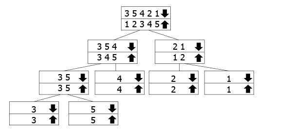
This tree is meant to represent how the recursive calls work. The arrays marked with the down arrow are the ones we call the function for, while we're merging the up arrow ones going back up. So you follow the down arrow to the bottom of the tree, and then go back up and merge.

In our example, we have the array 3 5 3 2 1, so we divide it into 3 5 4 and 2 1. To sort them, we further divide them into their components. Once we've reached the bottom, we start merging up and sorting them as we go.

If you'd like to read a detailed, dedicated article for Merge Sort, we've got you covered!

Implementation

The core function works pretty much as laid out in the explanation. We're just passing indexes left and right which are indexes of the leftmost and rightmost element of the subarray we want to sort. Initially, these should be 0 and array.length-1, depending on implementation.

The base of our recursion ensures we exit when we've finished, or when right and left meet each other. We find a midpoint mid, and sort subarrays left and right of it recursively, ultimately merging our solutions.

If you remember our tree graphic, you might wonder why we don't create two new smaller arrays and pass them on instead. This is because on really long arrays, this would cause huge memory consumption for something that's essentially unnecessary.

Merge Sort already doesn't work in-place because of the merge step, and this would only serve to worsen its memory efficiency. The logic of our tree of recursion otherwise stays the same, though, we just have to follow the indexes we're using:

public static void mergeSort(int[] array, int left, int right) {
    if (right <= left) return;
    int mid = (left+right)/2;
    mergeSort(array, left, mid);
    mergeSort(array, mid+1, right);
    merge(array, left, mid, right);
}

To merge the sorted subarrays into one, we'll need to calculate the length of each and make temporary arrays to copy them into, so we could freely change our main array.

After copying, we go through the resulting array and assign it the current minimum. Because our subarrays are sorted, we just chose the lesser of the two elements that haven't been chosen so far, and move the iterator for that subarray forward:

 void merge(int[] array, int left, int mid, int right) {
    // calculating lengths
    int lengthLeft = mid - left + 1;
    int lengthRight = right - mid;

    // creating temporary subarrays
    int leftArray[] = new int [lengthLeft];
    int rightArray[] = new int [lengthRight];

    // copying our sorted subarrays into temporaries
    for (int i = 0; i < lengthLeft; i++)
        leftArray[i] = array[left+i];
    for (int i = 0; i < lengthRight; i++)
        rightArray[i] = array[mid+i+1];

    // iterators containing current index of temp subarrays
    int leftIndex = 0;
    int rightIndex = 0;

    // copying from leftArray and rightArray back into array
    for (int i = left; i < right + 1; i++) {
        // if there are still uncopied elements in R and L, copy minimum of the two
        if (leftIndex < lengthLeft && rightIndex < lengthRight) {
            if (leftArray[leftIndex] < rightArray[rightIndex]) {
                array[i] = leftArray[leftIndex];
                leftIndex++;
            }
            else {
                array[i] = rightArray[rightIndex];
                rightIndex++;
            }
        }
        // if all the elements have been copied from rightArray, copy the rest of leftArray
        else if (leftIndex < lengthLeft) {
            array[i] = leftArray[leftIndex];
            leftIndex++;
        }
        // if all the elements have been copied from leftArray, copy the rest of rightArray
        else if (rightIndex < lengthRight) {
            array[i] = rightArray[rightIndex];
            rightIndex++;
        }
    }
}

Time Complexity

If we want to derive the complexity of recursive algorithms, we're going to have to get a little bit mathy.

The Master Theorem is used to figure out time complexity of recursive algorithms. For non-recursive algorithms, we could usually write the precise time complexity as some sort of an equation, and then we use Big-O Notation to sort them into classes of similarly-behaving algorithms.

The problem with recursive algorithms is that that same equation would look something like this:

$$
T(n) = aT(\frac{n}{b}) + cn^k
$$

The equation itself is recursive! In this equation, a tells us how many times we call the recursion, and b tells us how many parts our problem is divided into. In this case that may seem like an unimportant distinction because they're equal for merge sort, but for some problems they may not be.

The rest of the equation is the complexity of merging all of those solutions into one at the end. The Master Theorem solves this equation for us:

$$
T(n) = \Bigg\{
\begin{matrix}
O(n^{log_ba}), & a>b^k \\ O(n^klog n), & a = b^k \\ O(n^k), & a < b^k
\end{matrix}
$$

If T(n) is the runtime of the algorithm when sorting an array of the length n, Merge Sort would run twice for arrays that are half the length of the original array.

So if we have a=2, b=2. The merge step takes O(n) memory, so k=1. This means the equation for Merge Sort would look as follows:

$$
T(n) = 2T(\frac{n}{2})+cn
$$

If we apply The Master Theorem, we'll see that our case is the one where a=b^k because we have 2=2^1. That means our complexity is O(nlog n). This is an extremely good time complexity for a sorting algorithm, since it has been proven that an array can't be sorted any faster than O(nlog n).

While the version we've showcased is memory-consuming, there are more complex versions of Merge Sort that take up only O(1) space.

In addition, the algorithm is extremely easy to parallelize, since recursive calls from one node can be run completely independently from separate branches. While we won't be getting into how and why, as it's beyond the scope of this article, it's worth keeping in mind the pros of using this particular algorithm.

Heap Sort

Explanation

To properly understand why Heap Sort works, you must first understand the structure it's based on - the heap. We'll be talking in terms of a binary heap specifically, but you can generalize most of this to other heap structures as well.

A heap is a tree that satisfies the heap property, which is that for each node, all of its children are in a given relation to it. Additionally, a heap must be almost complete. An almost complete binary tree of depth d has a subtree of depth d-1 with the same root that is complete, and in which each node with a left descendent has a complete left subtree. In other words, when adding a node, we always go for the leftmost position in the highest incomplete level.

If the heap is a max-heap, then all of the children are smaller than the parent, and if it's a min-heap all of them are larger.

In other words, as you move down the tree, you get to smaller and smaller numbers (min-heap) or greater and greater numbers (max-heap). Here's an example of a max-heap:

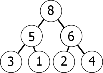
We can represent this max-heap in memory as an array in the following way:

8 5 6 3 1 2 4

You can envision it as reading from the graph level by level, left to right. What we have achieved by this is that if we take the kth element in the array, its children's positions are 2*k+1 and 2*k+2 (assuming the indexing starts at 0). You can check this for yourself.

Conversely, for the kth element the parent's position is always (k-1)/2.

Knowing this, you can easily "max-heapify" any given array. For each element, check if any of its children are smaller than it. If they are, swap one of them with the parent, and recursively repeat this step with the parent (because the new large element might still be bigger than its other child).

Leaves have no children, so they're trivially max-heaps of their own:

• 6 1 8 3 5 2 4: Both children are smaller than the parent, so everything stays the same.

• 6 1 8 3 5 2 4: Because 5 > 1, we swap them. We recursively heapify() for 5 now.

• 6 5 8 3 1 2 4: Both of the children are smaller, so nothing happens.

• 6 5 8 3 1 2 4: Because 8 > 6, we swap them.

• 8 5 6 3 1 2 4: We got the heap pictured above!

Once we've learned to heapify() an array the rest is pretty simple. We swap the root of the heap with the end of the array, and shorten the array by one.

We heapify() the shortened array again, and repeat the process:

• 8 5 6 3 1 2 4

• 4 5 6 3 1 2 8: swapped

• 6 5 4 3 1 2 8: heapified

• 2 5 4 3 1 6 8: swapped

• 5 2 4 2 1 6 8: heapified

• 1 2 4 2 5 6 8: swapped

And so on, I'm sure you can see the pattern emerging.

Implementation

static void heapify(int[] array, int length, int i) {
    int leftChild = 2*i+1;
    int rightChild = 2*i+2;
    int largest = i;

    // if the left child is larger than parent
    if (leftChild < length && array[leftChild] > array[largest]) {
        largest = leftChild;
    }

    // if the right child is larger than parent
    if (rightChild < length && array[rightChild] > array[largest]) {
        largest = rightChild;
    }

    // if a swap needs to occur
    if (largest != i) {
        int temp = array[i];
        array[i] = array[largest];
        array[largest] = temp;
        heapify(array, length, largest);
    }
}

public static void heapSort(int[] array) {
    if (array.length == 0) return;

    // Building the heap
    int length = array.length;
    // we're going from the first non-leaf to the root
    for (int i = length / 2-1; i >= 0; i--)
        heapify(array, length, i);

    for (int i = length-1; i >= 0; i--) {
        int temp = array[0];
        array[0] = array[i];
        array[i] = temp;

        heapify(array, i, 0);
    }
}

Time Complexity

When we look at the heapify() function, everything seems to be done in O(1), but then there's that pesky recursive call.

How many times will that be called, in the worst case scenario? Well, worst-case, it will propagate all the way to the top of the heap. It will do that by jumping to the parent of each node, so around the position i/2. that means it will make at worst log n jumps before it reaches the top, so the complexity is O(log n).

Because heapSort() is clearly O(n) due to for-loops iterating through the entire array, this would make the total complexity of Heap Sort O(nlog n).

Heap Sort is an in-place sort, meaning it takes O(1) additional space, as opposed to Merge Sort, but it has some drawbacks as well, such as being difficult to parallelize.

Quicksort

Explanation

Quicksort is another Divide and Conquer algorithm. It picks one element of an array as the pivot and sorts all of the other elements around it, for example smaller elements to the left, and larger to the right.

This guarantees that the pivot is in its proper place after the process. Then the algorithm recursively does the same for the left and right portions of the array.

Implementation

static int partition(int[] array, int begin, int end) {
    int pivot = end;

    int counter = begin;
    for (int i = begin; i < end; i++) {
        if (array[i] < array[pivot]) {
            int temp = array[counter];
            array[counter] = array[i];
            array[i] = temp;
            counter++;
        }
    }
    int temp = array[pivot];
    array[pivot] = array[counter];
    array[counter] = temp;

    return counter;
}

public static void quickSort(int[] array, int begin, int end) {
    if (end <= begin) return;
    int pivot = partition(array, begin, end);
    quickSort(array, begin, pivot-1);
    quickSort(array, pivot+1, end);
}

Time Complexity

The time complexity of Quicksort can be expressed with the following equation:

$$
T(n) = T(k) + T(n-k-1) + O(n)
$$

The worst case scenario is when the biggest or smallest element is always picked for pivot. The equation would then look like this:

$$
T(n) = T(0) + T(n-1) + O(n) = T(n-1) + O(n)
$$

This turns out to be O(n^2).

This may sound bad, as we have already learned multiple algorithms which run in O(nlog n) time as their worst case, but Quicksort is actually very widely used.

This is because it has a really good average runtime, also bounded by O(nlog n), and is very efficient for a large portion of possible inputs.

One of the reasons it is preferred to Merge Sort is that it doesn't take any extra space, all of the sorting is done in-place, and there's no expensive allocation and deallocation calls.

Performance Comparison

That all being said, it's often useful to run all of these algorithms on your machine a few times to get an idea of how they perform.

They'll perform differently with different collections that are being sorted of course, but even with that in mind, you should be able to notice some trends.

Let's run all of the implementations, one by one, each on a copy of a shuffled array of 10,000 integers:

time(ns)	Bubble Sort	Insertion Sort	Selection Sort	MergeSort	HeapSort	QuickSort
First Run	266,089,476	21,973,989	66,603,076	5,511,069	5,283,411	4,156,005
Second Run	323,692,591	29,138,068	80,963,267	8,075,023	6,420,768	7,060,203
Third Run	303,853,052	21,380,896	91,810,620	7,765,258	8,009,711	7,622,817
Fourth Run	410,171,593	30,995,411	96,545,412	6,560,722	5,837,317	2,358,377
Fifth Run	315,602,328	26,119,110	95,742,699	5,471,260	14,629,836	3,331,834
Sixth Run	286,841,514	26,789,954	90,266,152	9,898,465	4,671,969	4,401,080
Seventh Run	384,841,823	18,979,289	72,569,462	5,135,060	10,348,805	4,982,666
Eight Run	393,849,249	34,476,528	107,951,645	8,436,103	10,142,295	13,678,772
Ninth Run	306,140,830	57,831,705	138,244,799	5,154,343	5,654,133	4,663,260
Tenth Run	306,686,339	34,594,400	89,442,602	5,601,573	4,675,390	3,148,027

We can evidently see that Bubble Sort is the worst when it comes to performance. Avoid using it in production if you can't guarantee that it'll handle only small collections and it won't stall the application.

Heap Sort and Quick Sort are the best performance-wise. Although they're outputting similar results, QuickSort tends to be a bit better and more consistent - which checks out.

Sorting in Java

Comparable Interface

If you have your own types, it may get cumbersome implementing a separate sorting algorithm for each one. That's why Java provides an interface allowing you to use Collections.sort() on your own classes.

To do this, your class must implement the Comparable<T> interface, where T is your type, and override a method called .compareTo().

This method returns a negative integer if this is smaller than the argument element, 0 if they're equal, and a positive integer if this is greater.

In our example, we've made a class Student, and each student is identified by an id and a year they started their studies.

We want to sort them primarily by generations, but also secondarily by IDs:

public static class Student implements Comparable<Student> {
    int studentId;
    int studentGeneration;

    public Student(int studentId, int studentGeneration) {
        this.studentId = studentId;
        this.studentGeneration = studentGeneration;
    }

    @Override
    public String toString() {
        return studentId + "/" + studentGeneration % 100;
    }

    @Override
    public int compareTo(Student student) {
        int result = this.studentGeneration - student.studentGeneration;
        if (result != 0)
            return result;
        else
            return this.studentId - student.studentId;
    }
}

And here's how to use it in an application:

public static void main(String[] args) {
    Student[] a = new SortingAlgorithms.Student[5];
    a[0] = new Student(75, 2016);
    a[1] = new Student(52, 2019);
    a[2] = new Student(57, 2016);
    a[3] = new Student(220, 2014);
    a[4] = new Student(16, 2018);

    Arrays.sort(a);

    System.out.println(Arrays.toString(a));
}

Output:

[220/14, 57/16, 75/16, 16/18, 52/19]

Comparator Interface

We might want to sort our objects in an unorthodox way for a specific purpose, but we don't want to implement that as the default behavior of our class, or we might be sorting a collection of a built-in type in a non-default way.

For this, we can use the Comparator interface. For example, let's take our Student class, and sort only by ID:

public static class SortByID implements Comparator<Student> {
    public int compare(Student a, Student b) {
        return a.studentId - b.studentId;
    }
}

If we replace the sort call in main with the following:

Arrays.sort(a, new SortByID());

Output:

[16/18, 52/19, 57/16, 75/16, 220/14]

How it All Works

Collection.sort() works by calling the underlying Arrays.sort() method, while the sorting itself uses Insertion Sort for arrays shorter than 47, and Quicksort for the rest.

It's based on a specific two-pivot implementation of Quicksort which ensures it avoids most of the typical causes of degradation into quadratic performance, according to the JDK10 documentation.

Conclusion

Sorting is a very common operation with datasets, whether it is to analyze them further, speed up search by using more efficient algorithms that rely on the data being sorted, filter data, etc.

Sorting is supported by many languages and the interfaces often obscure what's actually happening to the programmer. While this abstraction is welcome and necessary for effective work, it can sometimes be deadly for efficiency, and it's good to know how to implement various algorithms and be familiar with their pros and cons, as well as how to easily access built-in implementations.