Statistical Hypothesis Analysis in Python with ANOVAs, Chi-Square, and Pearson Correlation

Introduction

Python is an incredibly versatile language, useful for a wide variety of tasks in a wide range of disciplines. One such discipline is statistical analysis on datasets, and along with SPSS, Python is one of the most common tools for statistics.

Python's user-friendly and intuitive nature makes running statistical tests and implementing analytical techniques easy, especially through the use of the statsmodels library.

Introducing the statsmodels Library in Python

The statsmodels library is a module for Python that gives easy access to a variety of statistical tools for carrying out statistical tests and exploring data. There are a number of statistical tests and functions that the library grants access to, including ordinary least squares (OLS) regressions, generalized linear models, logit models, Principal Component Analysis (PCA), and Autoregressive Integrated Moving Average (ARIMA) models.

The results of the models are constantly tested against other statistical packages to ensure that the models are accurate. When combined with SciPy and Pandas, it's simple to visualize data, run statistical tests, and check relationships for significance.

Choosing a Dataset

Before we can practice statistics with Python, we need to select a dataset. We'll be making use of a dataset compiled by the Gapminder Foundation.

The Gapminder Dataset tracks many variables used to assess the general health and wellness of populations in countries around the world. We'll be using the dataset because it is very well documented, standardized, and complete. We won't have to do much in the way of preprocessing in order to make use of it.

There are a few things we'll want to do just to get the dataset ready to run regressions, ANOVAs, and other tests, but by and large the dataset is ready to work with.

The starting point for our statistical analysis of the Gapminder dataset is exploratory data analysis. We'll use some graphing and plotting functions from Matplotlib and Seaborn to visualize some interesting relationships and get an idea of what variable relationships we may want to explore.

Exploratory Data Analysis and Preprocessing

We'll start off by visualizing some possible relationships. Using Seaborn and Pandas we can do some regressions that look at the strength of correlations between the variables in our dataset to get an idea of which variable relationships are worth studying.

We'll import those two and any other libraries we'll be using here:

import statsmodels.formula.api as smf
import statsmodels.stats.multicomp as multi
import scipy
from scipy.stats import pearsonr
import pandas as pd
from seaborn import regplot
import matplotlib.pyplot as plt
import numpy as np
import seaborn as sns

There isn't much preprocessing we have to do, but we do need to do a few things. First, we'll check for any missing or null data and convert any non-numeric entries to numeric. We'll also make a copy of the transformed dataframe that we'll work with:

# Check for missing data
def check_missing_values(df, cols):
    for col in cols:
        print("Column {} is missing:".format(col))
        print((df[col].values == ' ').sum())
        print()

# Convert to numeric
def convert_numeric(dataframe, cols):
    for col in cols:
        dataframe[col] = pd.to_numeric(dataframe[col], errors='coerce')

df = pd.read_csv("gapminder.csv")

print("Null values:")
print(df.isnull().values.any())

cols = ['lifeexpectancy', 'breastcancerper100th', 'suicideper100th']
norm_cols = ['internetuserate', 'employrate']

df2 = df.copy()

check_missing_values(df, cols)
check_missing_values(df, norm_cols)

convert_numeric(df2, cols)
convert_numeric(df2, norm_cols)

Here are the outputs:

Null values:
Column lifeexpectancy is missing:
22

Column breastcancerper100th is missing:
40

Column suicideper100th is missing:
22

Column internetuserate is missing:
21

Column employrate is missing:
35

There's a handful of missing values, but our numeric conversion should turn them into NaN values, allowing exploratory data analysis to be carried out on the dataset.

Specifically, we could try analyzing the relationship between internet use rate and life expectancy, or between internet use rate and employment rate. Let's try making individual graphs of some of these relationships using Seaborn and Matplotlib:

sns.lmplot(x="internetuserate", y="breastcancerper100th", data=df2, fit_reg=False)
plt.title("Internet Use Rate and Breast Cancer Per 100k")
plt.show()

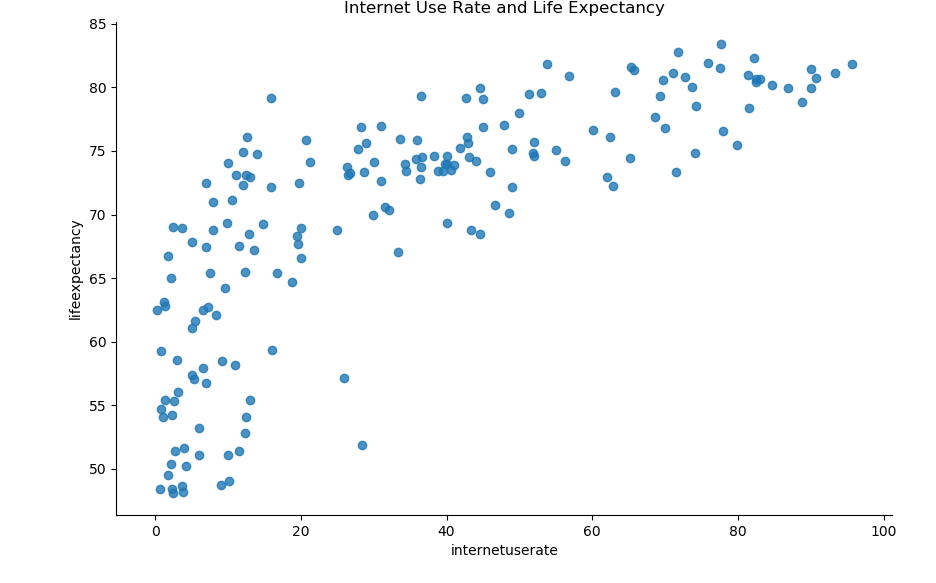
sns.lmplot(x="internetuserate", y="lifeexpectancy", data=df2, fit_reg=False)
plt.title("Internet Use Rate and Life Expectancy")
plt.show()

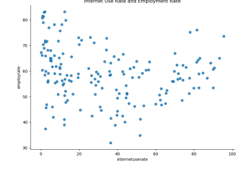
sns.lmplot(x="internetuserate", y="employrate", data=df2, fit_reg=False)
plt.title("Internet Use Rate and Employment Rate")
plt.show()

Here are the results of the graphs:

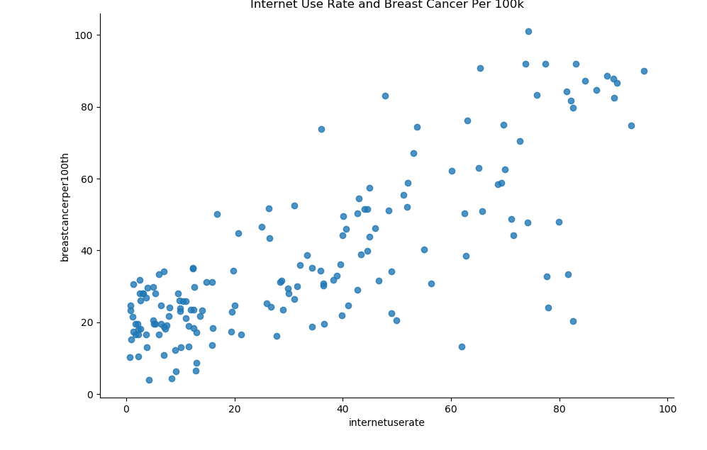
It looks like there are some interesting relationships that we could further investigate. Interestingly, there seems to be a fairly strong positive relationship between internet use rate and breast cancer, though this is likely just an artifact of better testing in countries that have more access to technology.

There also seems to be a fairly strong, though less linear relationship between life expectancy and internet use rate.

Finally, it looks like there is a parabolic, non-linear relationship between internet use rate and employment rate.

Selecting a Suitable Hypothesis

We want to pick out a relationship that merits further exploration. There are many potential relationships here that we could form a hypothesis about and explore the relationship with statistical tests. When we make a hypothesis and run a correlation test between the two variables, if the correlation test is significant, we then need to conduct statistical tests to see just how strong the correlation is and if we can reliably say that the correlation between the two variables is more than just chance.

The type of statistical test we use will depend on the nature of our explanatory and response variables, also known and independent and dependent variables. We'll go over how to run three different types of statistical tests:

• ANOVAs
• Chi-Square Tests
• Regressions.

We'll go with what we visualized above and choose to explore the relationship between internet use rates and life expectancy.

The null hypothesis is that there is no significant relationship between internet use rate and life expectancy, while our hypothesis is that there is a relationship between the two variables.

We're going to be conducting various types of hypothesis tests on the dataset. The type of hypothesis test that we use is dependent on the nature of our explanatory and response variables. Different combinations of explanatory and response variables require different statistical tests. For example, if one variable is categorical and one variable is quantitative in nature, an Analysis of Variance is required.

Analysis of Variance (ANOVA)

An Analysis of Variance (ANOVA) is a statistical test employed to compare two or more means together, which are determined through the analysis of variance. One-way ANOVA tests are utilized to analyze differences between groups and determine if the differences are statistically significant.

One-way ANOVAs compare two or more independent group means, though in practice they are most often used when there are at least three independent groups.

In order to carry out an ANOVA on the Gapminder dataset, we'll need to transform some of the features, as these values in the dataset are continuous but ANOVA analyses are appropriate for situations where one variable is categorical and one variable is quantitative.

We can transform the data from continuous to quantitative by selecting a category and binning the variable in question, dividing it into percentiles. The independent variable will be converted into a categorical variable, while the dependent variable will stay continuous. We can use the qcut() function in Pandas to divide the dataframe into bins:

def bin(dataframe, cols):
    # Create new columns that store the binned data
    for col in cols:
        new_col_name = "{}_bins".format(col)
        dataframe[new_col_name] = pd.qcut(dataframe[col], 10, labels=["1=10%", "2=20%", "3=30%", "4=40%", "5=50%", "6=60%", "7=70%", "8=80", "9=90%", "10=100%"])

df3 = df2.copy()

# This creates new columns filled with the binned column data
bin(df3, cols)
bin(df3, norm_cols)

After the variables have been transformed and are ready to be analyzed, we can use the statsmodel library to carry out an ANOVA on the selected features. We'll print out the results of the ANOVA and check to see if the relationship between the two variables is statistically significant:

anova_df = df3[['lifeexpectancy', 'internetuserate_bins', 'employrate_bins']].dropna()

relate_df = df3[['lifeexpectancy', 'internetuserate_bins']]

anova = smf.ols(formula='lifeexpectancy ~ C(internetuserate_bins)', data=anova_df).fit()

print(anova.summary())

# We may also want to check the mean and standard deviation for the groups
mean = relate_df.groupby("internetuserate_bins").mean()
sd = relate_df.groupby("internetuserate_bins").std()
print(mean)
print(sd)

Here's the output of the model:

                            OLS Regression Results                            
==============================================================================
Dep. Variable:         lifeexpectancy   R-squared:                       0.689
Model:                            OLS   Adj. R-squared:                  0.671
Method:                 Least Squares   F-statistic:                     38.65
Date:                Mon, 11 May 2020   Prob (F-statistic):           1.71e-35
Time:                        17:49:24   Log-Likelihood:                -521.54
No. Observations:                 167   AIC:                             1063.
Df Residuals:                     157   BIC:                             1094.
Df Model:                           9                                         
Covariance Type:            nonrobust                                         
======================================================================================================
                                         coef    std err          t      P>|t|      [0.025      0.975]
------------------------------------------------------------------------------------------------------
Intercept                             56.6603      1.268     44.700      0.000      54.157      59.164
C(internetuserate_bins)[T.2=20%]       1.6785      1.870      0.898      0.371      -2.015       5.372
C(internetuserate_bins)[T.3=30%]       5.5273      1.901      2.907      0.004       1.772       9.283
C(internetuserate_bins)[T.4=40%]      11.5693      1.842      6.282      0.000       7.932      15.207
C(internetuserate_bins)[T.5=50%]      14.6991      1.870      7.860      0.000      11.005      18.393
C(internetuserate_bins)[T.6=60%]      16.7287      1.870      8.946      0.000      13.035      20.422
C(internetuserate_bins)[T.7=70%]      17.8802      1.975      9.052      0.000      13.978      21.782
C(internetuserate_bins)[T.8=80]       19.8302      1.901     10.430      0.000      16.075      23.586
C(internetuserate_bins)[T.9=90%]      23.0723      1.901     12.135      0.000      19.317      26.828
C(internetuserate_bins)[T.10=100%]    23.3042      1.901     12.257      0.000      19.549      27.060
==============================================================================
Omnibus:                       10.625   Durbin-Watson:                   1.920
Prob(Omnibus):                  0.005   Jarque-Bera (JB):               11.911
Skew:                          -0.484   Prob(JB):                      0.00259
Kurtosis:                       3.879   Cond. No.                         10.0
==============================================================================

Warnings:
[1] Standard Errors assume that the covariance matrix of the errors is correctly specified.

We can see that the model gives a very small P-value (Prob F-statistic) of 1.71e-35. This is far less than the usual significance threshold of 0.05, so we conclude there is a significant relationship between life expectancy and internet use rate.

Since the correlation P-value does seem to be significant, and since we have 10 different categories, we'll want to run a post-hoc test to check that the difference between the means is still significant even after we check for type-1 errors. We can carry out post-hoc tests with the help of the multicomp module, utilizing a Tukey Honestly Significant Difference (Tukey HSD) test:

multi_comparison = multi.MultiComparison(anova_df["lifeexpectancy"], anova_df["internetuserate_bins"])
results = multi_comparison.tukeyhsd()
print(results)

Here are the results of the test:

  Multiple Comparison of Means - Tukey HSD, FWER=0.05  
=======================================================
 group1 group2 meandiff p-adj   lower    upper   reject
-------------------------------------------------------
10=100%  1=10% -23.3042  0.001 -29.4069 -17.2015   True
10=100%  2=20% -21.6257  0.001 -27.9633 -15.2882   True
10=100%  3=30% -17.7769  0.001 -24.2097  -11.344   True
10=100%  4=40% -11.7349  0.001 -17.9865  -5.4833   True
10=100%  5=50%  -8.6051  0.001 -14.9426  -2.2676   True
10=100%  6=60%  -6.5755 0.0352  -12.913   -0.238   True
10=100%  7=70%  -5.4241 0.2199 -12.0827   1.2346  False
10=100%   8=80  -3.4741 0.7474  -9.9069   2.9588  False
10=100%  9=90%  -0.2319    0.9  -6.6647    6.201  False
  1=10%  2=20%   1.6785    0.9  -4.3237   7.6807  False
  1=10%  3=30%   5.5273 0.1127  -0.5754  11.6301  False
  1=10%  4=40%  11.5693  0.001   5.6579  17.4807   True
  1=10%  5=50%  14.6991  0.001   8.6969  20.7013   True
  1=10%  6=60%  16.7287  0.001  10.7265  22.7309   True
  1=10%  7=70%  17.8801  0.001  11.5399  24.2204   True
  1=10%   8=80  19.8301  0.001  13.7274  25.9329   True
  1=10%  9=90%  23.0723  0.001  16.9696  29.1751   True
  2=20%  3=30%   3.8489 0.6171  -2.4887  10.1864  False
  2=20%  4=40%   9.8908  0.001   3.7374  16.0443   True
  2=20%  5=50%  13.0206  0.001   6.7799  19.2614   True
  2=20%  6=60%  15.0502  0.001   8.8095   21.291   True
  2=20%  7=70%  16.2017  0.001   9.6351  22.7683   True
  2=20%   8=80  18.1517  0.001  11.8141  24.4892   True
  2=20%  9=90%  21.3939  0.001  15.0563  27.7314   True
  3=30%  4=40%    6.042 0.0678  -0.2096  12.2936  False
  3=30%  5=50%   9.1718  0.001   2.8342  15.5093   True
  3=30%  6=60%  11.2014  0.001   4.8638  17.5389   True
  3=30%  7=70%  12.3528  0.001   5.6942  19.0114   True
  3=30%   8=80  14.3028  0.001     7.87  20.7357   True
  3=30%  9=90%   17.545  0.001  11.1122  23.9778   True
  4=40%  5=50%   3.1298 0.8083  -3.0237   9.2833  False
  4=40%  6=60%   5.1594 0.1862  -0.9941  11.3129  False
  4=40%  7=70%   6.3108 0.0638  -0.1729  12.7945  False
  4=40%   8=80   8.2608 0.0015   2.0092  14.5124   True
  4=40%  9=90%   11.503  0.001   5.2514  17.7546   True
  5=50%  6=60%   2.0296    0.9  -4.2112   8.2704  False
  5=50%  7=70%    3.181 0.8552  -3.3856   9.7476  False
  5=50%   8=80    5.131 0.2273  -1.2065  11.4686  False
  5=50%  9=90%   8.3732 0.0015   2.0357  14.7108   True
  6=60%  7=70%   1.1514    0.9  -5.4152    7.718  False
  6=60%   8=80   3.1014 0.8456  -3.2361    9.439  False
  6=60%  9=90%   6.3436 0.0496   0.0061  12.6812   True
  7=70%   8=80     1.95    0.9  -4.7086   8.6086  False
  7=70%  9=90%   5.1922 0.2754  -1.4664  11.8508  False
   8=80  9=90%   3.2422 0.8173  -3.1907    9.675  False
-------------------------------------------------------

Now we have some better insight into which groups in our comparison have statistically significant differences.

If the reject column has a label of False, we know it's recommended that we reject the null hypothesis and assume that there is a significant difference between the two groups being compared.

The Chi-Square Test of Independence

ANOVA is appropriate for instances where one variable is continuous and the other is categorical. Now we'll be looking at how to carry out a Chi-Square test of independence.

The Chi-Square test of independence is utilized when both explanatory and response variables are categorical. You likely also want to use the Chi-Square test when the explanatory variable is quantitative and the response variable is categorical, which you can do by dividing the explanatory variable into categories.

The Chi-Square test of independence is a statistical test used to analyze how significant a relationship between two categorical variables is. When a Chi-Square test is run, every category in one variable has its frequency compared against the second variable's categories. This means that the data can be displayed as a frequency table, where the rows represent the independent variables and the columns represent the dependent variables.

Much like we converted our independent variable into a categorical variable (by binning it), for the ANOVA test, we need to make both variables categorical in order to carry out the Chi-Square test. Our hypothesis for this problem is the same as the hypothesis in the previous problem, that there is a significant relationship between life expectancy and internet use rate.

We'll keep things simple for now and divide our internet use rate variable into two categories, though we could easily do more. We'll write a function to handle that.

We'll be conducting post-hoc comparison to guard against type-1 errors (false positives) using an approach called the Bonferroni Adjustment. In order to do this, you can carry out comparisons for the different possible pairs of your response variable, and then you check their adjusted significance.

We won't run comparisons for all the different possible pairs here, we'll just show how it can be done. We'll make a few different comparisons using a re-coding scheme and map the records into new feature columns.

Afterwards, we can check the observed counts and create tables of those comparisons:

def half_bin(dataframe, cols):
    for col in cols:
        new_col_name = "{}_bins_2".format(col)
        dataframe[new_col_name] = pd.qcut(dataframe[col], 2, labels=["1=50%", "2=100%"])

half_bin(df3, ['internetuserate'])

# Recoding scheme
recode_2 = {"3=30%": "3=30%", "7=70%": "7=70%"}
recode_3 = {"2=20%": "2=20%", "8=80": "8=80"}
recode_4 = {"6=60%": "6=60%", "9=90%": "9=90%"}
recode_5 = {"4=40%": "4=40%", "7=70%": "7=70%"}

# Create the new features
df3['Comp_3v7'] = df3['lifeexpectancy_bins'].map(recode_2)
df3['Comp_2v8'] = df3['lifeexpectancy_bins'].map(recode_3)
df3['Comp_6v9'] = df3['lifeexpectancy_bins'].map(recode_4)
df3['Comp_4v7'] = df3['lifeexpectancy_bins'].map(recode_5)

Running a Chi-Square test and post-hoc comparison involves first constructing a cross-tabs comparison table. The cross-tabs comparison table shows the percentage of occurrence for the response variable for the different levels of the explanatory variable.

Just to get an idea of how this works, let's print out the results for all the life expectancy bin comparisons:

# Get table of observed counts
count_table = pd.crosstab(df3['internetuserate_bins_2'], df3['lifeexpectancy_bins'])
print(count_table)

lifeexpectancy_bins     1=10%  2=20%  3=30%  4=40%  ...  7=70%  8=80  9=90%  10=100%
internetuserate_bins_2                              ...                             
1=50%                      18     19     16     14  ...      4     4      1        0
2=100%                      0      0      1      4  ...     15    11     16       19

We can see that a cross-tab comparison checks for the frequency of one variable's categories in the second variable. Above we see the distribution of life expectancies in situations where they fall into one of the two bins we created.

Now we need to compute the cross-tabs for the different pairs we created above, as this is what we run through the Chi-Square test:

count_table_3 = pd.crosstab(df3['internetuserate_bins_2'], df3['Comp_3v7'])
count_table_4 = pd.crosstab(df3['internetuserate_bins_2'], df3['Comp_2v8'])
count_table_5 = pd.crosstab(df3['internetuserate_bins_2'], df3['Comp_6v9'])
count_table_6 = pd.crosstab(df3['internetuserate_bins_2'], df3['Comp_4v7'])

Once we have transformed the variables so that the Chi-Square test can be carried out, we can use the chi2_contingency function in statsmodel to carry out the test.

We want to print out the column percentages as well as the results of the Chi-Square test, and we'll create a function to do this. We'll then use our function to do the Chi-Square test for the four comparison tables we created:

def chi_sq_test(table):
    print("Results for:")
    print(str(table))

    # Get column percentages
    col_sum = table.sum(axis=0)
    col_percents = table/col_sum
    print(col_percents)

    chi_square = scipy.stats.chi2_contingency(table)
    print("Chi-square value, p-value, expected_counts")
    print(chi_square)

    print()

print("Initial Chi-square:")
chi_sq_test(count_table)
print(" ")

chi_sq_test(count_table_3)
chi_sq_test(count_table_4)
chi_sq_test(count_table_5)
chi_sq_test(count_table_6)

Here are the results:

Initial Chi-square:
Results for:
lifeexpectancy_bins     1=10%  2=20%  3=30%  4=40%  ...  7=70%  8=80  9=90%  10=100%
internetuserate_bins_2                              ...                             
1=50%                      18     19     16     14  ...      4     4      1        0
2=100%                      0      0      1      4  ...     15    11     16       19

[2 rows x 10 columns]
lifeexpectancy_bins     1=10%  2=20%     3=30%  ...      8=80     9=90%  10=100%
internetuserate_bins_2                          ...                             
1=50%                     1.0    1.0  0.941176  ...  0.266667  0.058824      0.0
2=100%                    0.0    0.0  0.058824  ...  0.733333  0.941176      1.0

[2 rows x 10 columns]
Chi-square value, p-value, expected_counts
(102.04563740451277, 6.064860600653971e-18, 9, array([[9.45251397, 9.97765363, 8.9273743 , 9.45251397, 9.45251397,
        9.97765363, 9.97765363, 7.87709497, 8.9273743 , 9.97765363],
       [8.54748603, 9.02234637, 8.0726257 , 8.54748603, 8.54748603,
        9.02234637, 9.02234637, 7.12290503, 8.0726257 , 9.02234637]]))
-----
 
Results for:
Comp_3v7                3=30%  7=70%
internetuserate_bins_2              
1=50%                      16      4
2=100%                      1     15
Comp_3v7                   3=30%     7=70%
internetuserate_bins_2                    
1=50%                   0.941176  0.210526
2=100%                  0.058824  0.789474
Chi-square value, p-value, expected_counts
(16.55247678018576, 4.7322137795376575e-05, 1, array([[ 9.44444444, 10.55555556],
       [ 7.55555556,  8.44444444]]))
-----
Results for:
Comp_2v8                2=20%  8=80
internetuserate_bins_2             
1=50%                      19     4
2=100%                      0    11
Comp_2v8                2=20%      8=80
internetuserate_bins_2                 
1=50%                     1.0  0.266667
2=100%                    0.0  0.733333
Chi-square value, p-value, expected_counts
(17.382650301643437, 3.0560286589975315e-05, 1, array([[12.85294118, 10.14705882],
       [ 6.14705882,  4.85294118]]))
-----
Results for:
Comp_6v9                6=60%  9=90%
internetuserate_bins_2              
1=50%                       6      1
2=100%                     13     16
Comp_6v9                   6=60%     9=90%
internetuserate_bins_2                    
1=50%                   0.315789  0.058824
2=100%                  0.684211  0.941176
Chi-square value, p-value, expected_counts
(2.319693757720874, 0.12774517376836148, 1, array([[ 3.69444444,  3.30555556],
       [15.30555556, 13.69444444]]))
-----
Results for:
Comp_4v7                4=40%  7=70%
internetuserate_bins_2              
1=50%                      14      4
2=100%                      4     15
Comp_4v7                   4=40%     7=70%
internetuserate_bins_2                    
1=50%                   0.777778  0.210526
2=100%                  0.222222  0.789474
Chi-square value, p-value, expected_counts
(9.743247922437677, 0.0017998260000241526, 1, array([[8.75675676, 9.24324324],
       [9.24324324, 9.75675676]]))
-----

If we're only looking at the results for the full count table, it looks like there's a P-value of 6.064860600653971e-18.

However, in order to ascertain how the different groups diverge from one another, we need to carry out the Chi-Square test for the different pairs in our dataframe. We'll check to see if there is a statistically significant difference for each of the different pairs we selected. Note that the P-value which indicates a significant result changes depending on how many comparisons you are making, and while we won't cover that in this tutorial, you'll need to be mindful of it.

The 6 vs 9 comparison gives us a P-value of 0.127, which is above the 0.05 threshold, indicating that the difference for that category may be non-significant. Seeing the differences of the comparisons helps us understand why we need to compare different levels with one another.

Pearson Correlation

We've covered the test you should use when you have a categorical explanatory variable and a quantitative response variable (ANOVA), as well as the test you use when you have two categorical variables (Chi-Squared).

We'll now take a look at the appropriate type of test to use when you have a quantitative explanatory variable and a quantitative response variable - the Pearson Correlation.

The Pearson Correlation test is used to analyze the strength of a relationship between two provided variables, both quantitative in nature. The value, or strength of the Pearson correlation, will be between +1 and -1.

A correlation of 1 indicates a perfect association between the variables, and the correlation is either positive or negative. Correlation coefficients near 0 indicate very weak, almost non-existent, correlations. While there are other ways of measuring correlations between two variables, such as Spearman Correlation or Kendall Rank Correlation, the Pearson correlation is probably the most commonly used correlation test.

As the Gapminder dataset has its features represented with quantitative variables, we don't need to do any categorical transformation of the data before running a Pearson Correlation on it. Note that it's assumed that both variables are normally distributed and there aren't many significant outliers in the dataset. We'll need access to SciPy in order to carry out the Pearson correlation.

We'll graph the relationship between life expectancy and internet use rates, as well as internet use rate and employment rate, just to see what another correlation graph might look like. After creating a graphing function, we'll use the pearsonr() function from SciPy to carry out the correlation and check the results:

df_clean = df2.dropna()
df_clean['incomeperperson'] = df_clean['incomeperperson'].replace('', np.nan)

def plt_regression(x, y, data, label_1, label_2):
    reg_plot = regplot(x=x, y=y, fit_reg=True, data=data)
    plt.xlabel(label_1)
    plt.ylabel(label_2)
    plt.show()

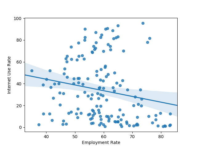
plt_regression('lifeexpectancy', 'internetuserate', df_clean, 'Life Expectancy', 'Internet Use Rate')
plt_regression('employrate', 'internetuserate', df_clean, 'Employment Rate', 'Internet Use Rate')

print('Assoc. - life expectancy and internet use rate')
print(pearsonr(df_clean['lifeexpectancy'], df_clean['internetuserate']))

print('Assoc. - between employment rate and internet use rate')
print(pearsonr(df_clean['employrate'], df_clean['internetuserate']))

Here are the outputs:

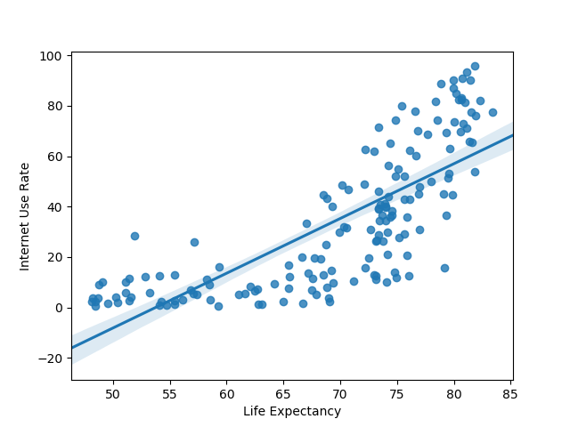
Assoc. - life expectancy and internet use rate
(0.77081050888289, 5.983388253650836e-33)
Assoc. - between employment rate and internet use rate
(-0.1950109538173115, 0.013175901971555317)

The first value is the direction and strength of the correlation, while the second is the P-value. The numbers suggest a fairly strong correlation between life expectancy and internet use rate that isn't due to chance. Meanwhile, there's a weaker, though still significant correlation between employment rate and internet use rate.

Note that it is also possible to run a Pearson Correlation on categorical data, though the results will look somewhat different. If we wanted to, we could group the income levels and run the Pearson Correlation on them. You can use it to check for the presence of moderating variables that could be having an effect on your association of interest.

Moderators and Statistical Interaction

Let's look at how to account for statistical interaction between multiple variables, AKA moderation.

Moderation is when a third (or more) variable impacts the strength of the association between the independent variable and the dependent variable.

There are different ways to test for moderation/statistical interaction between a third variable and the independent/dependent variables. For example, if you carried out an ANOVA test, you could test for moderation by doing a two-way ANOVA test in order to test for possible moderation.

However, a reliable way to test for moderation, no matter what type of statistical test you ran (ANOVA, Chi-Square, Pearson Correlation) is to check if there is an association between explanatory and response variables for every subgroup/level of the third variable.

To be more concrete, if you were carrying out ANOVA tests, you could just run an ANOVA for every category in the third variable (the variable you suspect might have a moderating effect on the relationship you are studying).

If you were using a Chi-Square test, you could just carry out a Chi-Square test on new dataframes holding all data points found within the categories of your moderating variable.

If your statistical test is a Pearson correlation, you would need to create categories or bins for the moderating variable and then run the Pearson correlation for all three of those bins.

Let's take a quick look at how to carry out Pearson Correlations for moderating variables. We'll create artificial categories/levels out of our continuous features. The process for testing for moderation for the other two test types (Chi-Square and ANOVA) is very similar, but you'll have pre-existing categorical variables to work with instead.

We'll want to choose a suitable variable to act as our moderating variable. Let's try income level per person and divide it into three different groups:

def income_groups(row):
    if row['incomeperperson'] <= 744.23:
        return 1
    elif row['incomeperperson'] <= 942.32:
        return 2
    else:
        return 3


# Apply function and set the new features in the dataframe
df_clean['income_group'] = df_clean.apply(lambda row: income_groups(row), axis=1)

# Create a few subframes to try test for moderation
subframe_1 = df_clean[(df_clean['income_group'] == 1)]
subframe_2 = df_clean[(df_clean['income_group'] == 2)]
subframe_3 = df_clean[(df_clean['income_group'] == 3)]

print('Assoc. - life expectancy and internet use rate for low income countries')

print(pearsonr(subframe_1['lifeexpectancy'], subframe_1['internetuserate']))

print('Assoc. - life expectancy and internet use rate for medium income countries')

print(pearsonr(subframe_2['lifeexpectancy'], subframe_2['internetuserate']))

print('Assoc. - life expectancy and internet use rate for high income countries')

print(pearsonr(subframe_3['lifeexpectancy'], subframe_3['internetuserate']))

Here are the outputs:

Assoc. - life expectancy and internet use rate for low income countries
(0.38386370068495235, 0.010101223355274047)

Assoc. - life expectancy and internet use rate for medium income countries
(0.9966009508278395, 0.05250454954743393)

Assoc. - life expectancy and internet use rate for high income countries
(0.7019997488251704, 6.526819886007788e-18)

Once more, the first value is the direction and strength of the correlation, while the second is the P-value.

Conclusion

statsmodels is an extremely useful library that allows Python users to analyze data and run statistical tests on datasets. You can carry out ANOVAs, Chi-Square Tests, Pearson Correlations and tests for moderation.

Once you become familiar with how to carry out these tests, you'll be able to test for significant relationships between dependent and independent variables, adapting for the categorical or continuous nature of the variables.