
Introduction
Preprocessing data is an often overlooked key step in Machine Learning. In fact - it's as important as the shiny model you want to fit with it.
Garbage in - garbage out.
You can have the best model crafted for any sort of problem - if you feed it garbage, it'll spew out garbage. It's worth noting that "garbage" doesn't refer to random data. It's a harsh label we attach to any data that doesn't allow the model to do its best - some more so than others. That being said - the same data can be bad for one model, but great for another. Generally, various Machine Learning models don't generalize as well on data with high scale variance, so you'll typically want to iron it out before feeding it into a model.
Normalization and Standardization are two techniques commonly used during Data Preprocessing to adjust the features to a common scale.
In this guide, we'll dive into what Feature Scaling is and scale the features of a dataset to a more fitting scale. Then, we'll train a SGDRegressor model on the original and scaled data to check whether it had much effect on this specific dataset.
What is Feature Scaling - Normalization and Standardization
Scaling or Feature Scaling is the process of changing the scale of certain features to a common one. This is typically achieved through normalization and standardization (scaling techniques).
- Normalization is the process of scaling data into a range of [0, 1]. It's more useful and common for regression tasks.
$$
x' = \frac{x-x_{min}}{x_{max} - x_{min}}
$$
- Standardization is the process of scaling data so that they have a mean value of 0 and a standard deviation of 1. It's more useful and common for classification tasks.
$$
x' = \frac{x-\mu}{\sigma}
$$
A normal distribution with these values is called a standard normal distribution.
It's worth noting that standardizing data doesn't guarantee that it'll be within the [0, 1] range. It most likely won't be - which can be a problem for certain algorithms that expect this range.
To perform standardization, Scikit-Learn provides us with the StandardScaler class.
Normalization is also known as Min-Max Scaling and Scikit-Learn provides the MinMaxScaler for this purpose. On the other hand, it also provides a Normalizer, which can make things a bit confusing.
Note: The Normalizer class doesn't perform the same scaling as MinMaxScaler. Normalizer works on rows, not features, and it scales them independently.
When to Perform Feature Scaling?
Feature Scaling doesn't guarantee better model performance for all models.
For instance, Feature Scaling doesn't do much if the scale doesn't matter. For K-Means Clustering, the Euclidean distance is important, so Feature Scaling makes a huge impact. It also makes a huge impact for any algorithms that rely on gradients, such as linear models that are fitted by minimizing loss with Gradient Descent.
Principal Component Analysis (PCA) also suffers from data that isn't scaled properly.
In the case of Scikit-Learn - you won't see any tangible difference with a LinearRegression, but will see a substantial difference with a SGDRegressor, because a SGDRegressor, which is also a linear model, depends on Stochastic Gradient Descent to fit the parameters.
A tree-based model won't suffer from unscaled data, because scale doesn't affect them at all, but if you perform Gradient Boosting on Classifiers, the scale does affect learning.
Importing Data and Exploratory Data Analysis
We'll be working with the Ames Housing Dataset which contains 79 features regarding houses sold in Ames, Iowa, as well as their sale price. This is a great dataset for basic and advanced regression training, since there are a lot of features to tweak and fiddle with, which ultimately usually affect the sales price in some way or the other.
Advice: If you'd like to dive deeper into an end-to-end regression project, check out our Guided Project: Hands-On House Price Prediction with Machine Learning in Python.
Let's import the data and take a look at some of the features we'll be using:
import pandas as pd
import matplotlib.pyplot as plt

# Load the Dataset
df = pd.read_csv('AmesHousing.csv')
# Single out a couple of predictor variables and labels ('SalePrice' is our target label set)
x = df[['Gr Liv Area', 'Overall Qual']].values
y = df['SalePrice'].values

fig, ax = plt.subplots(ncols=2, figsize=(12, 4))

ax[0].scatter(x[:,0], y)
ax[1].scatter(x[:,1], y)

plt.show()
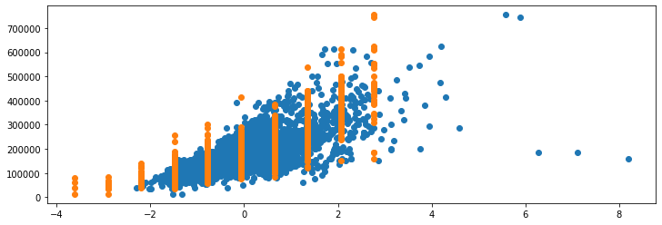
There's a clear strong positive correlation between the "Gr Liv Area" feature and the "SalePrice" feature - with only a couple of outliers. There's also a strong positive correlation between the "Overall Qual" feature and the "SalePrice":
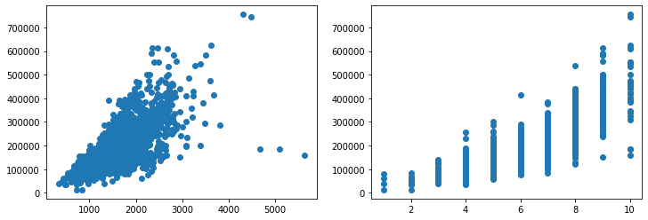
Though these are on a much different scale - the "Gr Liv Area" spans up to ~5000 (measured in square feet), while the "Overall Qual" feature spans up to 10 (discrete categories of quality). If we were to plot these two on the same axes, we wouldn't be able to tell much about the "Overall Qual" feature:
fig, ax = plt.subplots(figsize=(12, 4))

ax.scatter(x[:,0], y)
ax.scatter(x[:,1], y)
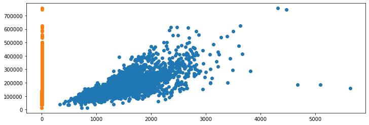
Additionally, if we were to plot their distributions, we wouldn't have much luck either:
fig, ax = plt.subplots(figsize=(12, 4))

ax.hist(x[:,0])
ax.hist(x[:,1])
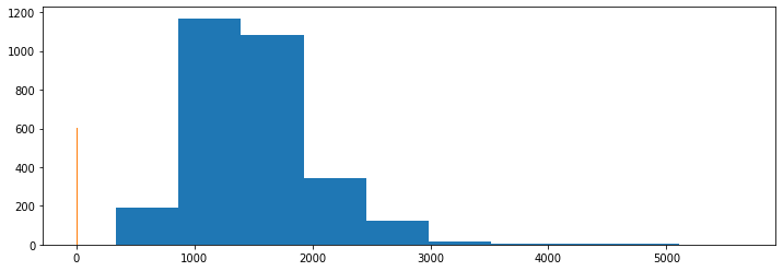
The scale of these features is so different that we can't really make much out by plotting them together. This is where feature scaling kicks in.
StandardScaler
The StandardScaler class is used to transform the data by standardizing it. Let's import it and scale the data via its fit_transform() method:
import pandas as pd
import matplotlib.pyplot as plt
# Import StandardScaler
from sklearn.preprocessing import StandardScaler

fig, ax = plt.subplots(figsize=(12, 4))

scaler = StandardScaler()
x_std = scaler.fit_transform(x)

ax.hist(x_std[:,0])
ax.hist(x_std[:,1])
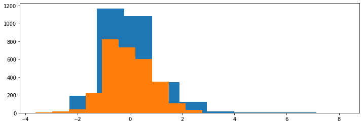
Note: We're using fit_transform() on the entirety of the dataset here to demonstrate the usage of the StandardScaler class and visualize its effects. When building a model or pipeline, like we will shortly - you shouldn't fit_transform() the entirety of the dataset, but rather, just fit() the training data, and transform() the testing data.
Running this piece of code will calculate the μ and σ parameters - this process is known as fitting the data, and then transform it so that these values correspond to 1 and 0 respectively.
When we plot the distributions of these features now, we'll be greeted with a much more manageable plot:
Check out our hands-on, practical guide to learning Git, with best-practices, industry-accepted standards, and included cheat sheet. Stop Googling Git commands and actually learn it!
If we were to plot these through Scatter Plots yet again, we'd perhaps more clearly see the effects of the standardization:
fig, ax = plt.subplots(figsize=(12, 4))

scaler = StandardScaler()
x_std = scaler.fit_transform(x)

ax.scatter(x_std[:,0], y)
ax.scatter(x_std[:,1], y)
MinMaxScaler
To normalize features, we use the MinMaxScaler class. It works in much the same way as StandardScaler, but uses a fundamentally different approach to scaling the data:
fig, ax = plt.subplots(figsize=(12, 4))

scaler = MinMaxScaler()
x_minmax = scaler.fit_transform(x)

ax.hist(x_minmax [:,0])
ax.hist(x_minmax [:,1])
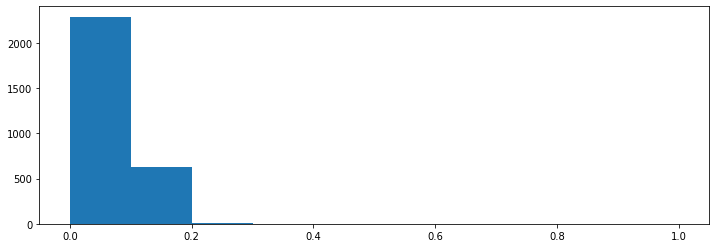
They are normalized in the range of [0, 1]. If we were to plot the distributions again, we'd be greeted with:
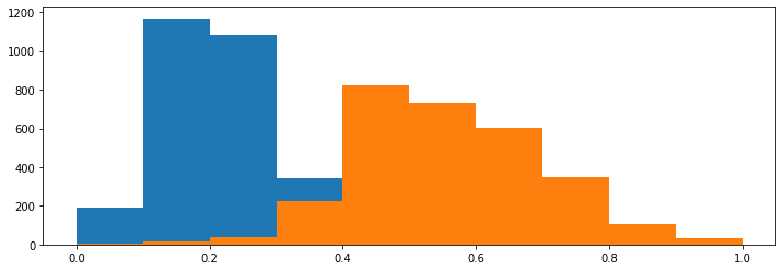
The skewness of the distribution is preserved, unlike with standardization which makes them overlap much more. Though, if we were to plot the data through Scatter Plots again:
fig, ax = plt.subplots(figsize=(12, 4))

scaler = MinMaxScaler()
x_minmax = scaler.fit_transform(x)

ax.scatter(x_minmax [:,0], y)
ax.scatter(x_minmax [:,1], y)
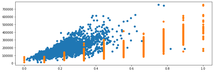
We'd be able to see the strong positive correlation between both of these with the "SalePrice" with the feature, but the "Overall Qual" feature awkwardly overextends to the right, because the outliers of the "Gr Liv Area" feature forced the majority of its distribution to trail on the left-hand side.
Effects of Outliers
Both normalization and standardization are sensitive to outliers - it's enough for the dataset to have a single outlier that's way out there to make things look really weird. Let's add a synthetic entry to the "Gr Liv Area" feature to see how it affects the scaling process:
fig, ax = plt.subplots(figsize=(12, 4))

scaler = MinMaxScaler()
x_minmax = scaler.fit_transform(x)

ax.scatter(x_minmax [:,0], y)
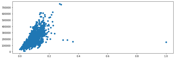
The single outlier, on the far right of the plot has really affected the new distribution. All of the data, except for the outlier is located in the first two quartiles:
fig, ax = plt.subplots(figsize=(12, 4))

scaler = MinMaxScaler()
x_minmax = scaler.fit_transform(x)

ax.hist(x_minmax [:,0])
Feature Scaling Through Scikit-Learn Pipelines
Finally, let's go ahead and train a model with and without scaling features beforehand. When working on Machine Learning projects - we typically have a pipeline for the data before it arrives at the model we're fitting.
We'll be using the Pipeline class which lets us minimize and, to a degree, automate this process, even though we have just two steps - scaling the data, and fitting a model:
from sklearn.model_selection import train_test_split
from sklearn.pipeline import Pipeline
from sklearn.linear_model import SGDRegressor
from sklearn.preprocessing import StandardScaler
from sklearn.preprocessing import MinMaxScaler
from sklearn.metrics import mean_absolute_error
import sklearn.metrics as metrics

import pandas as pd
import numpy as np
import matplotlib.pyplot as plt

# Import Data
df = pd.read_csv('AmesHousing.csv')
x = df[['Gr Liv Area', 'Overall Qual']].values
y = df['SalePrice'].values

# Split into a training and testing set
X_train, X_test, Y_train, Y_test = train_test_split(x, y)

# Define the pipeline for scaling and model fitting
pipeline = Pipeline([
    ("MinMax Scaling", MinMaxScaler()),
    ("SGD Regression", SGDRegressor())
])

# Scale the data and fit the model
pipeline.fit(X_train, Y_train)

# Evaluate the model
Y_pred = pipeline.predict(X_test)
print('Mean Absolute Error: ', mean_absolute_error(Y_pred, Y_test))
print('Score', pipeline.score(X_test, Y_test))
This results in:
Mean Absolute Error:  27614.031131858766
Score 0.7536086980531018
The mean absolute error is ~27000, and the accuracy score is ~75%. This means that on average, our model misses the price by $27000, which doesn't sound that bad, although it could be improved beyond this.
Most notably, the type of model we used is a bit too rigid and we haven't fed many features in so these two are most definitely the places that can be improved.
Though - let's not lose focus of what we're interested in. How does this model perform without Feature Scaling? Let's modify the pipeline to skip the scaling step:
pipeline = Pipeline([
    ("SGD Regression", SGDRegressor())
])
What happens might surprise you:
Mean Absolute Error:  1260383513716205.8
Score -2.772781517117743e+20
We've gone from ~75% accuracy to ~-3% accuracy just by skipping to scale our features. Any learning algorithm that depends on the scale of features will typically see major benefits from Feature Scaling. Those that don't, won't see much of a difference.
For instance, if we train a LinearRegression on this same data, with and without scaling, we'll see unremarkable results on the behalf of the scaling, and decent results on behalf of the model itself:
pipeline1 = Pipeline([
    ("Linear Regression", LinearRegression())
])

pipeline2 = Pipeline([
    ("Scaling", StandardScaler()),
    ("Linear Regression", LinearRegression())
])

pipeline1.fit(X_train, Y_train)
pipeline2.fit(X_train, Y_train)

Y_pred1 = pipeline1.predict(X_test)
Y_pred2 = pipeline2.predict(X_test)

print('Pipeline 1 Mean Absolute Error: ', mean_absolute_error(Y_pred1, Y_test))
print('Pipeline 1 Score', pipeline1.score(X_test, Y_test))

print('Pipeline 2 Mean Absolute Error: ', mean_absolute_error(Y_pred2, Y_test))
print('Pipeline 2 Score', pipeline2.score(X_test, Y_test))
Pipeline 1 Mean Absolute Error:  27706.61376199076
Pipeline 1 Score 0.7641840816646945

Pipeline 2 Mean Absolute Error:  27706.613761990764
Pipeline 2 Score 0.7641840816646945
Conclusion
Feature Scaling is the process of scaling the values of features to a more manageable scale. You'll typically perform it before feeding these features into algorithms that are affected by scale, during the preprocessing phase.
In this guide, we've taken a look at what Feature Scaling is and how to perform it in Python with Scikit-Learn, using StandardScaler to perform standardization and MinMaxScaler to perform normalization. We've also taken a look at how outliers affect these processes and the difference between a scale-sensitive model being trained with and without Feature Scaling.

