
After much hype, Google finally released TensorFlow 2.0 which is the latest version of Google's flagship deep learning platform. A lot of long-awaited features have been introduced in TensorFlow 2.0. This article very briefly covers how you can develop simple classification and regression models using TensorFlow 2.0.
Classification with Tensorflow 2.0
If you have ever worked with Keras library, you are in for a treat. TensorFlow 2.0 now uses Keras API as its default library for training classification and regression models. Before TensorFlow 2.0, one of the major criticisms that the earlier versions of TensorFlow had to face stemmed from the complexity of model creation. Previously you needed to stitch graphs, sessions and placeholders together in order to create even a simple logistic regression model. With TensorFlow 2.0, creating classification and regression models have become a piece of cake.
So without further ado, let's develop a classification model with TensorFlow.
The Dataset
The dataset for the classification example can be downloaded freely from this link. Download the file in CSV format. If you open the downloaded CSV file, you will see that the file doesn't contain any headers. The detail of the columns is available at UCI machine learning repository. I will recommend that you read the dataset information in detail from the download link. I will briefly summarize the dataset in this section.
The dataset basically consists of 7 columns:
- price (the buying price of the car)
- maint ( the maintenance cost)
- doors (number of doors)
- persons (the seating capacity)
- lug_capacity (the luggage capacity)
- safety (how safe is the car)
- output (the condition of the car)
Given the first 6 columns, the task is to predict the value for the 7th column i.e. the output. The output column can have one of the three values i.e. unacc (unacceptable), acc (acceptable), good, and very good.
Importing Libraries
Before we import the dataset into our application, we need to import the required libraries.
import pandas as pd
import numpy as np
import tensorflow as tf

import matplotlib.pyplot as plt
%matplotlib inline

import seaborn as sns
sns.set(style="darkgrid")
Before we proceed, I want you to make sure that you have the latest version of TensorFlow i.e. TensorFlow 2.0. You can check your TensorFlow version with the following command:
print(tf.__version__)
If you do not have TensorFlow 2.0 installed, you can upgrade to the latest version via the following command:
$ pip install --upgrade tensorflow
Importing the Dataset
The following script imports the dataset. Change the path to your CSV data file accordingly.
cols = ['price', 'maint', 'doors', 'persons', 'lug_capacity', 'safety','output']
cars = pd.read_csv(r'/content/drive/My Drive/datasets/car_dataset.csv', names=cols, header=None)
Since the CSV file doesn't contain column headers by default, we passed a list of column headers to the pd.read_csv() method.
Let's now see the first 5 rows of the dataset via the head() method.
cars.head()
Output:
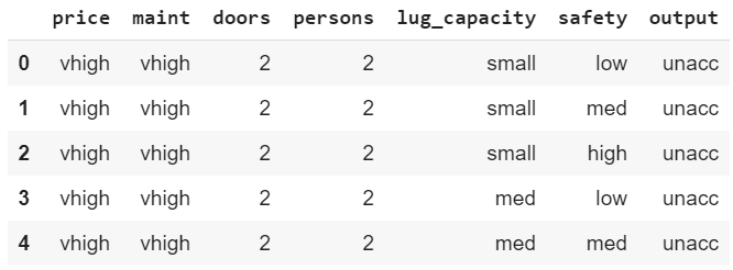
You can see the 7 columns in the dataset.
Data Analysis and Preprocessing
Let's briefly analyze the dataset by plotting a pie chart that shows the distribution of the output. The following script increases the default plot size.
plot_size = plt.rcParams["figure.figsize"]
plot_size [0] = 8
plot_size [1] = 6
plt.rcParams["figure.figsize"] = plot_size
And the following script plots the pie chart showing the output distribution.
cars.output.value_counts().plot(kind='pie', autopct='%0.05f%%', colors=['lightblue', 'lightgreen', 'orange', 'pink'], explode=(0.05, 0.05, 0.05,0.05))
Output:
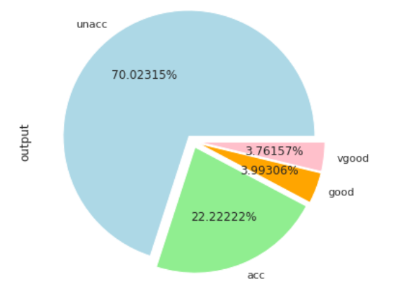
The output shows that the majority of cars (70%) are in unacceptable condition while 20% cars are in acceptable conditions. The ratio of cars in good and very good condition is very low.
All the columns in our dataset are categorical. Deep learning is based on statistical algorithms and statistical algorithms work with numbers. Therefore, we need to convert the categorical information into numeric columns. There are various approaches to do that but one of the most common approaches is one-hot encoding. In one-hot encoding, for each unique value in the categorical column, a new column is created. For the rows in the actual column where the unique value existed, a 1 is added to the corresponding row of the column created for that particular value. This might sound complex but the following example will make it clear.
The following script converts categorical columns into numeric columns:
price = pd.get_dummies(cars.price, prefix='price')
maint = pd.get_dummies(cars.maint, prefix='maint')

doors = pd.get_dummies(cars.doors, prefix='doors')
persons = pd.get_dummies(cars.persons, prefix='persons')

lug_capacity = pd.get_dummies(cars.lug_capacity, prefix='lug_capacity')
safety = pd.get_dummies(cars.safety, prefix='safety')

labels = pd.get_dummies(cars.output, prefix='condition')
To create our feature set, we can merge the first six columns horizontally:
X = pd.concat([price, maint, doors, persons, lug_capacity, safety] , axis=1)
Let's see how our label column looks now:
labels.head()
Output:
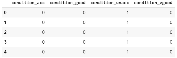
The label column is basically a one-hot encoded version of the output column that we had in our dataset. The output column had four unique values: unacc, acc, good and very good. In the one-hot encoded label dataset, you can see four columns, one for each of the unique values in the output column. You can see 1 in the column for the unique value that originally existed in that row. For instance, in the first five rows of the output column, the column value was unacc. In the labels column, you can see 1 in the first five rows of the condition_unacc column.
Let's now convert our labels into a NumPy array since deep learning models in TensorFlow accept NumPy arrays as input.
y = labels.values
The final step before we can train our TensorFlow 2.0 classification model is to divide the dataset into training and test sets:
from sklearn.model_selection import train_test_split
X_train, X_test, y_train, y_test = train_test_split(X, y, test_size=0.20, random_state=42)
Model Training
To train the model, let's import the TensorFlow 2.0 classes. Execute the following script:
Check out our hands-on, practical guide to learning Git, with best-practices, industry-accepted standards, and included cheat sheet. Stop Googling Git commands and actually learn it!
from tensorflow.keras.layers import Input, Dense, Activation,Dropout
from tensorflow.keras.models import Model
As I said earlier, TensorFlow 2.0 uses the Keras API for training the model. In the script above we basically import Input, Dense, Activation, and Dropout classes from the tensorflow.keras.layers module. Similarly, we also import the Model class from the tensorflow.keras.models module.
The next step is to create our classification model:
input_layer = Input(shape=(X.shape[1],))
dense_layer_1 = Dense(15, activation='relu')(input_layer)
dense_layer_2 = Dense(10, activation='relu')(dense_layer_1)
output = Dense(y.shape[1], activation='softmax')(dense_layer_2)

model = Model(inputs=input_layer, outputs=output)
model.compile(loss='categorical_crossentropy', optimizer='adam', metrics=['acc'])
As can be seen from the script, the model contains three dense layers. The first two dense layers contain 15 and 10 nodes, respectively with relu activation function. The final dense layer contains 4 nodes (y.shape[1] == 4) and a softmax activation function since this is a classification task. The model is trained using categorical_crossentropy loss function and adam optimizer. The evaluation metric is accuracy.
The following script shows the model summary:
print(model.summary())
Output:
Model: "model"
_________________________________________________________________
Layer (type)                 Output Shape              Param #
=================================================================
input_1 (InputLayer)         [(None, 21)]              0
_________________________________________________________________
dense (Dense)                (None, 15)                330
_________________________________________________________________
dense_1 (Dense)              (None, 10)                160
_________________________________________________________________
dense_2 (Dense)              (None, 4)                 44
=================================================================
Total params: 534
Trainable params: 534
Non-trainable params: 0
_________________________________________________________________
None
Finally, to train the model execute the following script:
history = model.fit(X_train, y_train, batch_size=8, epochs=50, verbose=1, validation_split=0.2)
The model will be trained for 50 epochs but here for the sake of space, the result of only last 5 epochs is displayed:
Epoch 45/50
1105/1105 [==============================] - 0s 219us/sample - loss: 0.0114 - acc: 1.0000 - val_loss: 0.0606 - val_acc: 0.9856
Epoch 46/50
1105/1105 [==============================] - 0s 212us/sample - loss: 0.0113 - acc: 1.0000 - val_loss: 0.0497 - val_acc: 0.9856
Epoch 47/50
1105/1105 [==============================] - 0s 219us/sample - loss: 0.0102 - acc: 1.0000 - val_loss: 0.0517 - val_acc: 0.9856
Epoch 48/50
1105/1105 [==============================] - 0s 218us/sample - loss: 0.0091 - acc: 1.0000 - val_loss: 0.0536 - val_acc: 0.9856
Epoch 49/50
1105/1105 [==============================] - 0s 213us/sample - loss: 0.0095 - acc: 1.0000 - val_loss: 0.0513 - val_acc: 0.9819
Epoch 50/50
1105/1105 [==============================] - 0s 209us/sample - loss: 0.0080 - acc: 1.0000 - val_loss: 0.0536 - val_acc: 0.9856
By the end of the 50th epoch, we have training accuracy of 100% while validation accuracy of 98.56%, which is impressive.
Let's finally evaluate the performance of our classification model on the test set:
score = model.evaluate(X_test, y_test, verbose=1)

print("Test Score:", score[0])
print("Test Accuracy:", score[1])
Here is the output:
WARNING:tensorflow:Falling back from v2 loop because of error: Failed to find data adapter that can handle input: <class 'pandas.core.frame.DataFrame'>, <class 'NoneType'>
346/346 [==============================] - 0s 55us/sample - loss: 0.0605 - acc: 0.9740
Test Score: 0.06045335989359314
Test Accuracy: 0.9739884
Our model achieves an accuracy of 97.39% on the test set. Though it is slightly less than the training accuracy of 100%, it is still very good given the fact that we randomly chose the number of layers and the nodes. You can add more layers to the model with more nodes and see if you can get better results on the validation and test sets.
Regression with TensorFlow 2.0
In a regression problem, the goal is to predict a continuous value. In this section, you will see how to solve a regression problem with TensorFlow 2.0
The Dataset
The dataset for this problem can be downloaded freely from this link. Download the CSV file.
The following script imports the dataset. Do not forget to change the path to your own CSV datafile.
petrol_cons = pd.read_csv(r'/content/drive/My Drive/datasets/petrol_consumption.csv')
Let's print the first five rows of the dataset via the head() function:
petrol_cons.head()
Output:
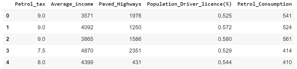
You can see that there are five columns in the dataset. The regression model will be trained on the first four columns, i.e. Petrol_tax, Average_income, Paved_Highways, and Population_Driver_License(%). The value for the last column i.e. Petrol_Consumption will be predicted. As you can see that there is no discrete value for the output column, rather the predicted value can be any continuous value.
Data Preprocessing
In the data preprocessing step we will simply split the data into features and labels, followed by dividing the data into test and training sets. Finally the data will be normalized. For regression problems in general, and for regression problems with deep learning, it is highly recommended that you normalize your dataset. Finally, since all the columns are numeric, here we do not need to perform one-hot encoding of the columns.
X = petrol_cons.iloc[:, 0:4].values
y = petrol_cons.iloc[:, 4].values

from sklearn.model_selection import train_test_split

X_train, X_test, y_train, y_test = train_test_split(X, y, test_size=0.2, random_state=0)

from sklearn.preprocessing import StandardScaler

sc = StandardScaler()
X_train = sc.fit_transform(X_train)
X_test = sc.transform(X_test)
In the above script, in the feature set X, the first four columns of the dataset are included. In the label set y, only the 5th column is included. Next, the data set is divided into training and test size via the train_test_split method of the sklearn.model_selection module. The value for the test_size attribute is 0.2 which means that the test set will contain 20% of the original data and the training set will consist of the remaining 80% of the original dataset. Finally, the StandardScaler class from the sklearn.preprocessing module is used to scale the dataset.
Model Training
The next step is to train our model. This process is quite similar to training the classification. The only change will be in the loss function and the number of nodes in the output dense layer. Since now we are predicting a single continuous value, the output layer will only have 1 node.
input_layer = Input(shape=(X.shape[1],))
dense_layer_1 = Dense(100, activation='relu')(input_layer)
dense_layer_2 = Dense(50, activation='relu')(dense_layer_1)
dense_layer_3 = Dense(25, activation='relu')(dense_layer_2)
output = Dense(1)(dense_layer_3)

model = Model(inputs=input_layer, outputs=output)
model.compile(loss="mean_squared_error" , optimizer="adam", metrics=["mean_squared_error"])
Our model consists of four dense layers with 100, 50, 25, and 1 node, respectively. For regression problems, one of the most commonly used loss functions is mean_squared_error. The following script prints the summary of the model:
Model: "model_2"
_________________________________________________________________
Layer (type)                 Output Shape              Param #
=================================================================
input_4 (InputLayer)         [(None, 4)]               0
_________________________________________________________________
dense_10 (Dense)             (None, 100)               500
_________________________________________________________________
dense_11 (Dense)             (None, 50)                5050
_________________________________________________________________
dense_12 (Dense)             (None, 25)                1275
_________________________________________________________________
dense_13 (Dense)             (None, 1)                 26
=================================================================
Total params: 6,851
Trainable params: 6,851
Non-trainable params: 0
Finally, we can train the model with the following script:
history = model.fit(X_train, y_train, batch_size=2, epochs=100, verbose=1, validation_split=0.2)
Here is the result from the last 5 training epochs:
Epoch 96/100
30/30 [==============================] - 0s 2ms/sample - loss: 510.3316 - mean_squared_error: 510.3317 - val_loss: 10383.5234 - val_mean_squared_error: 10383.5234
Epoch 97/100
30/30 [==============================] - 0s 2ms/sample - loss: 523.3454 - mean_squared_error: 523.3453 - val_loss: 10488.3036 - val_mean_squared_error: 10488.3037
Epoch 98/100
30/30 [==============================] - 0s 2ms/sample - loss: 514.8281 - mean_squared_error: 514.8281 - val_loss: 10379.5087 - val_mean_squared_error: 10379.5088
Epoch 99/100
30/30 [==============================] - 0s 2ms/sample - loss: 504.0919 - mean_squared_error: 504.0919 - val_loss: 10301.3304 - val_mean_squared_error: 10301.3311
Epoch 100/100
30/30 [==============================] - 0s 2ms/sample - loss: 532.7809 - mean_squared_error: 532.7809 - val_loss: 10325.1699 - val_mean_squared_error: 10325.1709
To evaluate the performance of a regression model on a test set, one of the most commonly used metrics is root mean squared error. We can find mean squared error between the predicted and actual values via the mean_squared_error class of the sklearn.metrics module. We can then take the square root of the resultant mean squared error. Look at the following script:
from sklearn.metrics import mean_squared_error
from math import sqrt

pred_train = model.predict(X_train)
print(np.sqrt(mean_squared_error(y_train,pred_train)))

pred = model.predict(X_test)
print(np.sqrt(mean_squared_error(y_test,pred)))
The output shows the mean squared error for both the training and test sets. The results show that model performance is better on the training set since the root mean squared error value for the training set is less. Our model is overfitting. The reason is obvious, we only had 48 records in the dataset. Try to train regression models with a larger dataset to get better results.
50.43599665058207
84.31961060849562
Conclusion
TensorFlow 2.0 is the latest version of Google's TensorFlow library for deep learning. This article briefly covers how to create classification and regression models with TensorFlow 2.0. To have hands-on experience, I would suggest that you practice the examples given in this article and try to create simple regression and classification models with TensorFlow 2.0 using some other datasets.

