
This is the first article in the series of articles on "Creating a Neural Network From Scratch in Python".
- Creating a Neural Network from Scratch in Python
- Creating a Neural Network from Scratch in Python: Adding Hidden Layers
- Creating a Neural Network from Scratch in Python: Multi-class Classification
Introduction
Have you ever wondered how chat-bots like Siri, Alexa, and Cortana are able to respond to user queries? Or how autonomous cars are able to drive themselves without any human help? All of these fancy products have one thing in common: Artificial Intelligence (AI). It is the AI which enables them to perform such tasks without being supervised or controlled by a human. But the question remains: "What is AI?" A simple answer to this question is: "AI is a combination of complex algorithms from the various mathematical domains such as Algebra, Calculus, and Probability and Statistics."
In this article, we will study a simple artificial neural network, which is one of the main building blocks of artificial intelligence. Different variants of an Artificial Neural Network exist, dedicated to solving a particular problem. For instance Convolutional Neural Networks are commonly used for Image Recognition problems while Recurrent Neural Networks are used to solve sequence problems.
There are many deep learning libraries that can be used to create a neural network in a single line of code. However, if you really want to understand the in-depth working of a neural network, I suggest you learn how to code it from scratch in any programming language. Performing this exercise will really clear up many of the concepts for you. And this is exactly what we will do in this article.
The Problem
Since this is an introductory article, the problem that we are going to solve is pretty simple. Suppose we have some information about obesity, smoking habits, and exercise habits of five people. We also know whether these people are diabetic or not. Our dataset looks like this:
| Person | Smoking | Obesity | Exercise | Diabetic |
|---|---|---|---|---|
| Person 1 | 0 | 1 | 0 | 1 |
| Person 2 | 0 | 0 | 1 | 0 |
| Person 3 | 1 | 0 | 0 | 0 |
| Person 4 | 1 | 1 | 0 | 1 |
| Person 5 | 1 | 1 | 1 | 1 |
In the above table, we have five columns: Person, Smoking, Obesity, Exercise, and Diabetic. Here 1 refers to true and 0 refers to false. For instance, the first person has values of 0, 1, 0 which means that the person doesn't smoke, is obese, and doesn't exercise. The person is also diabetic.
It is clearly evident from the dataset that a person's obesity is indicative of him being diabetic. Our task is to create a neural network that is able to predict whether an unknown person is diabetic or not given data about his exercise habits, obesity, and smoking habits. This is a type of supervised learning problem where we are given inputs and corresponding correct outputs and our task is to find the mapping between the inputs and the outputs.
Note: This is just a fictional dataset, in real life, obese people are not necessarily always diabetic.
The Solution
We will create a very simple neural network with one input layer and one output layer. Before writing any actual code, let's first let's see how our neural network will execute, in theory.
Neural Network Theory
A neural network is a supervised learning algorithm which means that we provide the input data containing the independent variables and the output data that contains the dependent variable. For instance, in our example our independent variables are smoking, obesity and exercise. The dependent variable is whether a person is diabetic or not.
In the beginning, the neural network makes some random predictions, these predictions are matched with the correct output and the error or the difference between the predicted values and the actual values is calculated. The function that finds the difference between the actual value and the propagated values is called the cost function. The cost here refers to the error. Our objective is to minimize the cost function. Training a neural network basically refers to minimizing the cost function. We will see how we can perform this task.
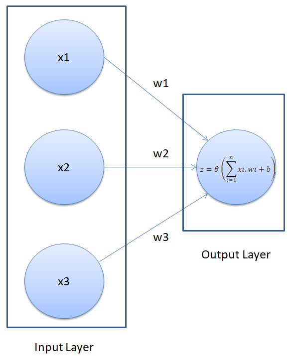
The neural network that we are going to create has the following visual representation.
A neural network executes in two steps: Feed Forward and Back Propagation. We will discuss both of these steps in detail.
Feed Forward
In the feed-forward part of a neural network, predictions are made based on the values in the input nodes and the weights. If you look at the neural network in the above figure, you will see that we have three features in the dataset: smoking, obesity, and exercise, therefore we have three nodes in the first layer, also known as the input layer. We have replaced our feature names with the variable x, for generality in the figure above.
The weights of a neural network are basically the strings that we have to adjust in order to be able to correctly predict our output. For now, just remember that for each input feature, we have one weight.
The following are the steps that execute during the feedforward phase of a neural network:
Step 1: (Calculate the dot product between inputs and weights)
The nodes in the input layer are connected with the output layer via three weight parameters. In the output layer, the values in the input nodes are multiplied with their corresponding weights and are added together. Finally, the bias term is added to the sum. The b in the above figure refers to the bias term.
The bias term is very important here. Suppose if we have a person who doesn't smoke, is not obese, and doesn't exercise, the sum of the products of input nodes and weights will be zero. In that case, the output will always be zero no matter how much we train the algorithms. Therefore, in order to be able to make predictions, even if we do not have any non-zero information about the person, we need a bias term. The bias term is necessary to make a robust neural network.
Mathematically, in step 1, we perform the following calculation:
$$
X.W = x1w1 + x2w2 + x3w3 + b
$$
Step 2: (Pass the result from step 1 through an activation function)
The result from Step 1 can be a set of any values. However, in our output we have the values in the form of 1 and 0. We want our output to be in the same format. To do so we need an activation function, which squashes input values between 1 and 0. One such activation function is the sigmoid function.
The sigmoid function returns 0.5 when the input is 0. It returns a value close to 1 if the input is a large positive number. In case of negative input, the sigmoid function outputs a value close to zero.
Mathematically, the sigmoid function can be represented as:
$$
\theta_{X.W} = \frac{\mathrm{1} }{\mathrm{1} + e^{-X.W} }
$$
Let us try to plot the sigmoid function:
input = np.linspace(-10, 10, 100)

def sigmoid(x):
    return 1/(1+np.exp(-x))

from matplotlib import pyplot as plt
plt.plot(input, sigmoid(input), c="r")
In the script above, we first randomly generate 100 linearly-spaced points between -10 and 10. To do so, we use the linspace method from the NumPy library. Next, we define the sigmoid function. Finally, we use the matplotlib library to plot the input values against the values returned by the sigmoid function. The output looks likes this:
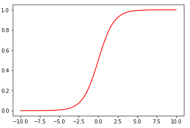
You can see that if the input is a negative number, the output is close to zero, otherwise if the input is positive the output is close to 1. However, the output is always between 0 and 1. This is what we want.
This sums up the feedforward part of our neural network. It is pretty straightforward. First we have to find the dot product of the input feature matrix with the weight matrix. Next, pass the result from the output through an activation function, which in this case is the sigmoid function. The result of the activation function is basically the predicted output for the input features.
Back Propagation
In the beginning, before you do any training, the neural network makes random predictions which are far from correct.
The principle behind the working of a neural network is simple. We start by letting the network make random predictions about the output. We then compare the predicted output of the neural network with the actual output. Next, we fine-tune our weights and the bias in such a manner that our predicted output becomes closer to the actual output, which is basically known as "training the neural network".
In the back propagation section, we train our algorithm. Let's take a look at the steps involved in the back propagation section.
Step 1: (Calculating the cost)
The first step in the back propagation section is to find the "cost" of the predictions. The cost of the prediction can simply be calculated by finding the difference between the predicted output and the actual output. The higher the difference, the higher the cost will be.
There are several other ways to find the cost, but we will use the mean squared error cost function. A cost function is simply the function that finds the cost of the given predictions.
The mean squared error cost function can be mathematically represented as:
$$
MSE =
\frac{\mathrm{1} }{\mathrm{n}}
\sum\nolimits_{i=1}^{n}
(predicted - observed)^{2}
$$
Here n is the number of observations.
Step 2: (Minimizing the cost)
Our ultimate purpose is to fine-tune the knobs of our neural network in such a way that the cost is minimized. If you look at our neural network, you'll notice that we can only control the weights and the bias. Everything else is beyond our control. We cannot control the inputs, we cannot control the dot products, and we cannot manipulate the sigmoid function.
In order to minimize the cost, we need to find the weight and bias values for which the cost function returns the smallest value possible. The smaller the cost, the more correct our predictions are.
This is an optimization problem where we have to find the function minima.
To find the minima of a function, we can use the gradient decent algorithm. The gradient descent algorithm can be mathematically represented as follows:
Here in the above equation, J is the cost function. Basically what the above equation says is: find the partial derivative of the cost function with respect to each weight and bias and subtract the result from the existing weight values to get the new weight values.
The derivative of a function gives us its slope at any given point. To find if the cost increases or decreases, given the weight value, we can find the derivative of the function at that particular weight value. If the cost increases with the increase in weight, the derivative will return a positive value which will then be subtracted from the existing value.
On the other hand, if the cost is decreasing with an increase in weight, a negative value will be returned, which will be added to the existing weight value since negative into negative is positive.
In Equation 1, we can see there is an alpha symbol, which is multiplied by the gradient. This is called the learning rate. The learning rate defines how fast our algorithm learns. For more details about how learning rate can be defined, check out this article .
We need to repeat the execution of Equation 1 for all the weights and bias until the cost is minimized to the desirable level. In other words, we need to keep executing Equation 1 until we get such values for bias and weights, for which the cost function returns a value close to zero.
And that's pretty much it. Now is the time to implement what we have studied so far. We will create a simple neural network with one input and one output layer in Python.
Neural Network Implementation in Python
Let's first create our feature set and the corresponding labels. Execute the following script:
import numpy as np
feature_set = np.array([[0,1,0],[0,0,1],[1,0,0],[1,1,0],[1,1,1]])
labels = np.array([[1,0,0,1,1]])
labels = labels.reshape(5,1)
In the above script, we create our feature set. It contains five records. Similarly, we created a labels set which contains corresponding labels for each record in the feature set. The labels are the answers we're trying to predict with the neural network.
The next step is to define hyper parameters for our neural network. Execute the following script to do so:
np.random.seed(42)
weights = np.random.rand(3,1)
bias = np.random.rand(1)
lr = 0.05
In the script above we used the random.seed function so that we can get the same random values whenever the script is executed.
In the next step, we initialize our weights with normally distributed random numbers. Since we have three features in the input, we have a vector of three weights. We then initialize the bias value with another random number. Finally, we set the learning rate to 0.05.
Next, we need to define our activation function and its derivative (I'll explain in a moment why we need to find the derivative of the activation). Our activation function is the sigmoid function, which we covered earlier.
Check out our hands-on, practical guide to learning Git, with best-practices, industry-accepted standards, and included cheat sheet. Stop Googling Git commands and actually learn it!
The following Python script creates this function:
def sigmoid(x):
    return 1/(1+np.exp(-x))
And the method that calculates the derivative of the sigmoid function is defined as follows:
def sigmoid_der(x):
    return sigmoid(x)*(1-sigmoid(x))
The derivative of sigmoid function is simply sigmoid(x) * sigmoid(1-x).
Now we are ready to train our neural network that will be able to predict whether a person is obese or not.
Look at the following script:
for epoch in range(20000):
    inputs = feature_set

    # feedforward step1
    XW = np.dot(feature_set, weights) + bias

    #feedforward step2
    z = sigmoid(XW)


    # backpropagation step 1
    error = z - labels

    print(error.sum())

    # backpropagation step 2
    dcost_dpred = error
    dpred_dz = sigmoid_der(z)

    z_delta = dcost_dpred * dpred_dz

    inputs = feature_set.T
    weights -= lr * np.dot(inputs, z_delta)

    for num in z_delta:
        bias -= lr * num
Don't get intimidated by this code. I will explain it line by line.
In the first step, we define the number of epochs. An epoch is basically the number of times we want to train the algorithm on our data. We will train the algorithm on our data 20,000 times. I have tested this number and found that the error is pretty much minimized after 20,000 iterations. You can try with a different number. The ultimate goal is to minimize the error.
Next we store the values from the feature_set to the input variable. We then execute the following line:
XW = np.dot(feature_set, weights) + bias
Here we find the dot product of the input and the weight vector and add bias to it. This is Step 1 of the feedforward section.
In this line:
z = sigmoid(XW)
We pass the dot product through the sigmoid activation function, as explained in Step 2 of the feedforward section. This completes the feed forward part of our algorithm.
Now is the time to start back-propagation. The variable z contains the predicted outputs. The first step of the back-propagation is to find the error. We do so in the following line:
error = z - labels
We then print the error on the screen.
Now is the time to execute Step 2 of back-propagation, which is the gist of this code.
We know that our cost function is:
$$
MSE = \frac{\mathrm{1} }{\mathrm{n}} \sum\nolimits_{i=1}^{n} (predicted - observed)^{2}
$$
We need to differentiate this function with respect to each weight. We will use the chain rule of differentiation for this purpose. Let's suppose "d_cost" is the derivate of our cost function with respect to weight "w", we can use chain rule to find this derivative, as shown below:
Here,
can be calculated as:
Here, 2 is constant and therefore can be ignored. This is basically the error which we already calculated. In the code, you can see the line:
dcost_dpred = error # ........ (2)
Next we have to find:
Here "d_pred" is simply the sigmoid function and we have differentiated it with respect to the input dot product "z". In the script, this is defined as:
dpred_dz = sigmoid_der(z) # ......... (3)
Finally, we have to find:
We know that:
Therefore, the derivative with respect to any weight is simply the corresponding input. Hence, our final derivative of the cost function with respect to any weight is:
slope = input x dcost_dpred x dpred_dz
Take a look at the following three lines:
z_delta = dcost_dpred * dpred_dz
inputs = feature_set.T
weights -= lr * np.dot(inputs, z_delta)
Here we have the z_delta variable, which contains the product of dcost_dpred and dpred_dz . Instead of looping through each record and multiplying the input with corresponding z_delta, we take the transpose of the input feature matrix and multiply it with the z_delta. Finally, we multiply the learning rate variable lr with the derivative to increase the speed of convergence.
We then looped through each derivative value and update our bias values, as well as shown in this script:
Once the loop starts, you will see that the total error starts decreasing as shown below:
0.001700995120272485
0.001700910187124885
0.0017008252625468727
0.0017007403465365955
0.00170065543909367
0.0017005705402162556
0.0017004856499031988
0.0017004007681529695
0.0017003158949647542
0.0017002310303364868
0.0017001461742678046
0.0017000613267565308
0.0016999764878018585
0.0016998916574025129
0.00169980683555691
0.0016997220222637836
0.0016996372175222992
0.0016995524213307602
0.0016994676336875778
0.0016993828545920908
0.0016992980840424554
0.0016992133220379794
0.0016991285685766487
0.0016990438236577712
0.0016989590872797753
0.0016988743594415108
0.0016987896401412066
0.0016987049293782815
You can see that error is extremely small at the end of the training of our neural network. At this point of time our weights and biases will have values that can be used to detect whether a person is diabetic or not, based on his smoking habits, obesity, and exercise habits.
You can now try and predict the value of a single instance. Let's suppose we have a record of a patient that comes in who smokes, is not obese, and doesn't exercise. Let's find out if he is likely to be diabetic or not. The input feature will look like this: [1,0,0].
Execute the following script:
single_point = np.array([1,0,0])
result = sigmoid(np.dot(single_point, weights) + bias)
print(result)
In the output you will see:
[0.00707584]
You can see that the person is likely not diabetic since the value is much closer to 0 than 1.
Now let's test another person who doesn't smoke, is obese, and doesn't exercise. The input feature vector will be [0,1,0]. Execute this script:
single_point = np.array([0,1,0])
result = sigmoid(np.dot(single_point, weights) + bias)
print(result)
In the output you will see the following value:
[0.99837029]
You can see that the value is very close to 1, which is likely due to the person's obesity.
Resources
Want to learn more about creating neural networks to solve complex problems? If so, try checking out some other resources, like this online course:
Deep Learning A-Z: Hands-On Artificial Neural Networks
It covers neural networks in much more detail, including convolutional neural networks, recurrent neural networks, and much more.
Conclusion
In this article we created a very simple neural network with one input and one output layer from scratch in Python. Such a neural network is simply called a perceptron. A perceptron is able to classify linearly separable data. Linearly separable data is the type of data which can be separated by a hyperplane in n-dimensional space.
Real-word artificial neural networks are much more complex, powerful, and consist of multiple hidden layers and multiple nodes in the hidden layer. Such neural networks are able to identify non-linear real decision boundaries. I will explain how to create a multi-layer neural network from scratch in Python in an upcoming article.

