Creating a Neural Network from Scratch in Python: Multi-class Classification

This is the third article in the series of articles on "Creating a Neural Network From Scratch in Python".

• Creating a Neural Network from Scratch in Python
• Creating a Neural Network from Scratch in Python: Adding Hidden Layers
• Creating a Neural Network from Scratch in Python: Multi-class Classification

If you have no prior experience with neural networks, I would suggest you first read Part 1 and Part 2 of the series (linked above). Once you feel comfortable with the concepts explained in those articles, you can come back and continue this article.

Introduction

In the previous article, we saw how we can create a neural network from scratch, which is capable of solving binary classification problems, in Python. A binary classification problem has only two outputs. However, real-world problems are far more complex.

Consider the example of the digit recognition problem where we use the image of a digit as an input and the classifier predicts the corresponding digit number. A digit can be any number between 0 and 9. This is a classic example of a multi-class classification problem where input may belong to any of the 10 possible outputs.

In this article, we will see how we can create a simple neural network from scratch in Python, which is capable of solving multi-class classification problems.

Dataset

Let's first briefly take a look at our dataset. Our dataset will have two input features and one of the three possible outputs. We will manually create a dataset for this article.

To do so, execute the following script:

import numpy as np
import matplotlib.pyplot as plt

np.random.seed(42)

cat_images = np.random.randn(700, 2) + np.array([0, -3])
mouse_images = np.random.randn(700, 2) + np.array([3, 3])
dog_images = np.random.randn(700, 2) + np.array([-3, 3])

In the script above, we start by importing our libraries and then we create three two-dimensional arrays of size 700 x 2. You can think of each element in one set of the array as an image of a particular animal. Each array element corresponds to one of the three output classes.

An important point to note here is that, if we plot the elements of the cat_images array on a two-dimensional plane, they will be centered around x=0 and y=-3. Similarly, the elements of the mouse_images array will be centered around x=3 and y=3, and finally, the elements of the array dog_images will be centered around x=-3 and y=3. You will see this once we plot our dataset.

Next, we need to vertically join these arrays to create our final dataset. Execute the following script to do so:

feature_set = np.vstack([cat_images, mouse_images, dog_images])

We created our feature set, and now we need to define corresponding labels for each record in our feature set. The following script does that:

labels = np.array([0]*700 + [1]*700 + [2]*700)

The above script creates a one-dimensional array of 2100 elements. The first 700 elements have been labeled as 0, the next 700 elements have been labeled as 1 while the last 700 elements have been labeled as 2. This is just our shortcut way of quickly creating the labels for our corresponding data.

For multi-class classification problems, we need to define the output label as a one-hot encoded vector since our output layer will have three nodes and each node will correspond to one output class. We want that when an output is predicted, the value of the corresponding node should be 1 while the remaining nodes should have a value of 0. For that, we need three values for the output label for each record. This is why we convert our output vector into a one-hot encoded vector.

Execute the following script to create the one-hot encoded vector array for our dataset:

one_hot_labels = np.zeros((2100, 3))

for i in range(2100):
    one_hot_labels[i, labels[i]] = 1

In the above script we create the one_hot_labels array of size 2100 x 3 where each row contains a one-hot encoded vector for the corresponding record in the feature set. We then insert 1 in the corresponding column.

If you execute the above script, you will see that the one_hot_labels array will have 1 at index 0 for the first 700 records, 1 at index 1 for next 700 records while 1 at index 2 for the last 700 records.

Now let's plot the dataset that we just created. Execute the following script:

plt.scatter(feature_set[:,0], feature_set[:,1], c=labels, cmap='plasma', s=100, alpha=0.5)
plt.show()

Once you execute the above script, you should see the following figure:

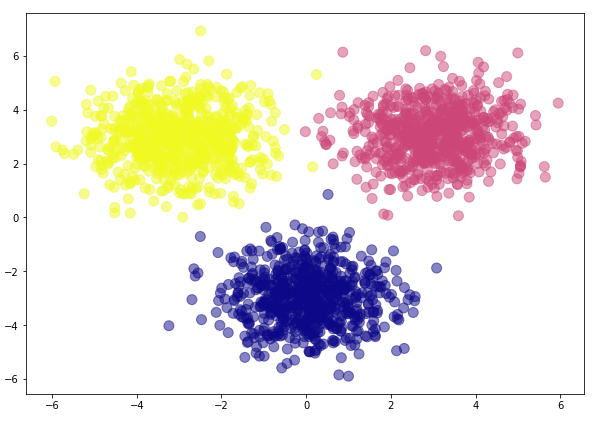
You can clearly see that we have elements belonging to three different classes. Our task will be to develop a neural network capable of classifying data into the aforementioned classes.

Neural Network with Multiple Output Classes

The neural network that we are going to design has the following architecture:

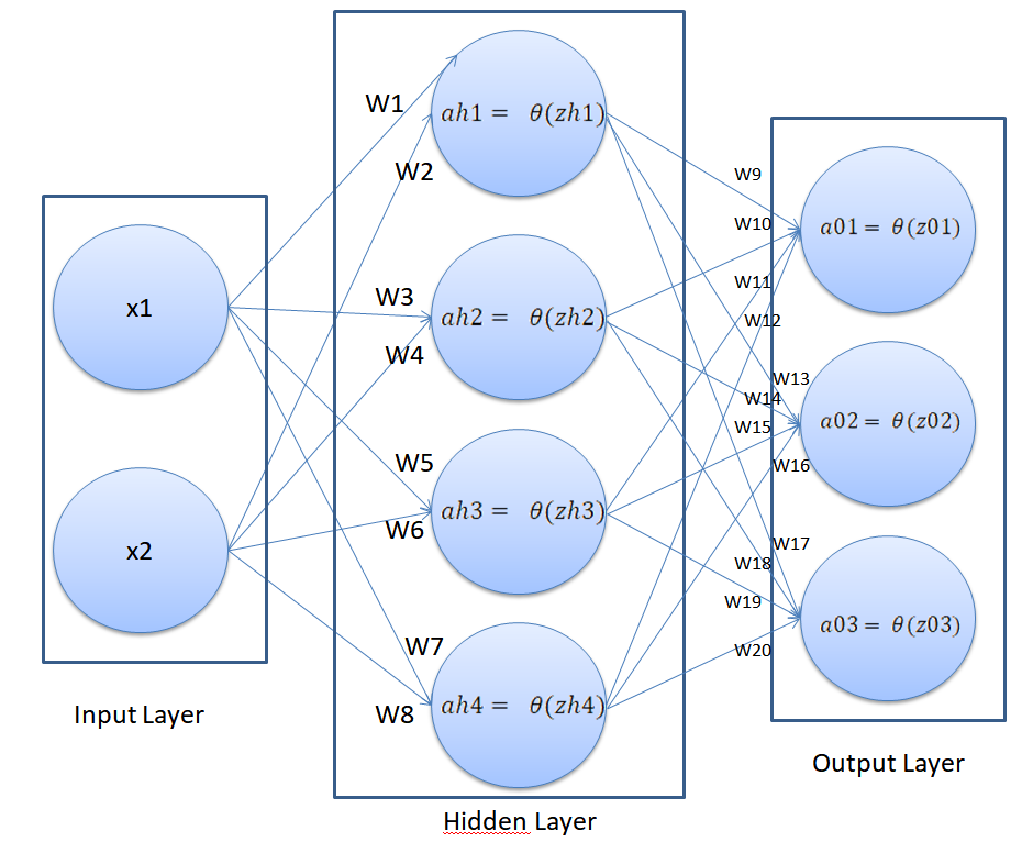
You can see that our neural network is pretty similar to the one we developed in Part 2 of the series. It has an input layer with 2 input features and a hidden layer with 4 nodes. However, in the output layer, we can see that we have three nodes. This means that our neural network is capable of solving the multi-class classification problem where the number of possible outputs is 3.

Softmax and Cross-Entropy Functions

Before we move on to the code section, let us briefly review the softmax and cross entropy functions, which are respectively the most commonly used activation and loss functions for creating a neural network for multi-class classification.

Softmax Function

From the architecture of our neural network, we can see that we have three nodes in the output layer. We have several options for the activation function at the output layer. One option is to use the sigmoid function as we did in the previous articles.

However, there is a more convenient activation function in the form of softmax that takes a vector as input and produces another vector of the same length as output. Since our output contains three nodes, we can consider the output from each node as one element of the input vector. The output will be a length of the same vector where the values of all the elements sum to 1. Mathematically, the softmax function can be represented as:

The softmax function simply divides the exponent of each input element by the sum of exponents of all the input elements. Let's take a look at a simple example of this:

def softmax(A):
    expA = np.exp(A)
    return expA / expA.sum()

nums = np.array([4, 5, 6])
print(softmax(nums))

In the script above we create a softmax function that takes a single vector as input, takes exponents of all the elements in the vector and then divides the resulting numbers individually by the sum of exponents of all the numbers in the input vector.

You can see that the input vector contains elements 4, 5 and 6. In the output, you will see three numbers squashed between 0 and 1 where the sum of the numbers will be equal to 1. The output looks likes this:

[0.09003057 0.24472847 0.66524096]

Softmax activation function has two major advantages over the other activation functions, particularly for multi-class classification problems: The first advantage is that softmax function takes a vector as input and the second advantage is that it produces an output between 0 and 1. Remember, in our dataset, we have one-hot encoded output labels which mean that our output will have values between 0 and 1. However, the output of the feed-forward process can be greater than 1, therefore softmax function is the ideal choice at the output layer since it squashes the output between 0 and 1.

Cross-Entropy Function

With softmax activation function at the output layer, mean squared error cost function can be used for optimizing the cost as we did in the previous articles. However, for the softmax function, a more convenient cost function exists which is called cross-entropy.

Mathematically, the cross-entropy function looks likes this:

The cross-entropy is simply the sum of the products of all the actual probabilities with the negative log of the predicted probabilities. For multi-class classification problems, the cross-entropy function is known to outperform the gradient descent function.

Now we have sufficient knowledge to create a neural network that solves multi-class classification problems. Let's see how our neural network will work.

As always, a neural network executes in two steps: Feed-forward and back-propagation.

Feed Forward

The feed-forward phase will remain more or less similar to what we saw in the previous article. The only difference is that now we will use the softmax activation function at the output layer rather than sigmoid function.

Remember, for the hidden layer output we will still use the sigmoid function as we did previously. The softmax function will be used only for the output layer activations.

Phase 1

Since we are using two different activation functions for the hidden layer and the output layer, I have divided the feed-forward phase into two sub-phases.

In the first phase, we will see how to calculate output from the hidden layer. For each input record, we have two features "x1" and "x2". To calculate the output values for each node in the hidden layer, we have to multiply the input with the corresponding weights of the hidden layer node for which we are calculating the value. Notice, we are also adding a bias term here. We then pass the dot product through the sigmoid activation function to get the final value.

For instance to calculate the final value for the first node in the hidden layer, which is denoted by "ah1", you need to perform the following calculation:

$$
zh1 = x1w1 + x2w2 + b
$$

$$
ah1 = \frac{\mathrm{1} }{\mathrm{1} + e^{-zh1} }
$$

This is the resulting value for the top-most node in the hidden layer. In the same way, you can calculate the values for the 2nd, 3rd, and 4th nodes of the hidden layer.

Phase 2

To calculate the values for the output layer, the values in the hidden layer nodes are treated as inputs. Therefore, to calculate the output, multiply the values of the hidden layer nodes with their corresponding weights and pass the result through an activation function, which will be softmax in this case.

This operation can be mathematically expressed by the following equation:

$$
zo1 = ah1w9 + ah2w10 + ah3w11 + ah4w12
$$

$$
zo2 = ah1w13 + ah2w14 + ah3w15 + ah4w16
$$

$$
zo3 = ah1w17 + ah2w18 + ah3w19 + ah4w20
$$

Here zo1, zo2, and zo3 will form the vector that we will use as input to the sigmoid function. Let's name this vector "zo".

zo = [zo1, zo2, zo3]

Now to find the output value a01, we can use softmax function as follows:

$$
ao1(zo) = \frac{e^{zo1}}{ \sum\nolimits_{k=1}^{k}{e^{zok}} }
$$

Here "a01" is the output for the top-most node in the output layer. In the same way, you can use the softmax function to calculate the values for ao2 and ao3.

You can see that the feed-forward step for a neural network with multi-class output is pretty similar to the feed-forward step of the neural network for binary classification problems. The only difference is that here we are using the softmax function at the output layer rather than the sigmoid function.

Back-Propagation

The basic idea behind back-propagation remains the same. We have to define a cost function and then optimize that cost function by updating the weights such that the cost is minimized. However, unlike previous articles where we used mean squared error as a cost function, in this article we will instead use cross-entropy function.

Back-propagation is an optimization problem where we have to find the function minima for our cost function.

To find the minima of a function, we can use the gradient decent algorithm. The gradient descent algorithm can be mathematically represented as follows:

The details regarding how gradient descent function minimizes the cost have already been discussed in the previous article. Here we'll just see the mathematical operations that we need to perform.

Our cost function is:

In our neural network, we have an output vector where each element of the vector corresponds to output from one node in the output layer. The output vector is calculated using the softmax function. If "ao" is the vector of the predicted outputs from all output nodes and "y" is the vector of the actual outputs of the corresponding nodes in the output vector, we have to basically minimize this function:

Phase 1

In the first phase, we need to update weights w9 up to w20. These are the weights of the output layer nodes.

From the previous article, we know that to minimize the cost function, we have to update weight values such that the cost decreases. To do so, we need to take the derivative of the cost function with respect to each weight. Mathematically we can represent it as:

$$
\frac {dcost}{dwo} = \frac {dcost}{dao} *, \frac {dao}{dzo} * \frac {dzo}{dwo} ..... (1)
$$

Here "wo" refers to the weights in the output layer.

The first part of the equation can be represented as:

$$
\frac {dcost}{dao} *\ \frac {dao}{dzo} ....... (2)
$$

The detailed derivation of cross-entropy loss function with softmax activation function can be found at this link.

The derivative of equation (2) is:

$$
\frac {dcost}{dao} *\ \frac {dao}{dzo} = ao - y ....... (3)
$$

Where "ao" is the predicted output while "y" is the actual output.

Finally, we need to find "dzo" with respect to "dwo" from Equation 1. The derivative is simply the outputs coming from the hidden layer as shown below:

$$
\frac {dzo}{dwo} = ah
$$

To find new weight values, the values returned by Equation 1 can be simply multiplied with the learning rate and subtracted from the current weight values.

We also need to update the bias "bo" for the output layer. We need to differentiate our cost function with respect to bias to get new bias value as shown below:

$$
\frac {dcost}{dbo} = \frac {dcost}{dao} *\ \frac {dao}{dzo} * \frac {dzo}{dbo} ..... (4)
$$

The first part of the Equation 4 has already been calculated in Equation 3. Here we only need to update "dzo" with respect to "bo" which is simply 1. So:

$$
\frac {dcost}{dbo} = ao - y ........... (5)
$$

To find new bias values for the output layer, the values returned by Equation 5 can be simply multiplied with the learning rate and subtracted from the current bias value.

Phase 2

In this section, we will back-propagate our error to the previous layer and find the new weight values for hidden layer weights i.e. weights w1 to w8.

Let's collectively denote hidden layer weights as "wh". We basically have to differentiate the cost function with respect to "wh".

Mathematically we can use chain rule of differentiation to represent it as:

$$
\frac {dcost}{dwh} = \frac {dcost}{dah} *, \frac {dah}{dzh} * \frac {dzh}{dwh} ...... (6)
$$

Here again, we will break Equation 6 into individual terms.

The first term "dcost" can be differentiated with respect to "dah" using the chain rule of differentiation as follows:

$$
\frac {dcost}{dah} = \frac {dcost}{dzo} *\ \frac {dzo}{dah} ...... (7)
$$

Let's again break the Equation 7 into individual terms. From the Equation 3, we know that:

$$
\frac {dcost}{dao} *\ \frac {dao}{dzo} =\frac {dcost}{dzo} = = ao - y ........ (8)
$$

Now we need to find dzo/dah from Equation 7, which is equal to the weights of the output layer as shown below:

$$
\frac {dzo}{dah} = wo ...... (9)
$$

Now we can find the value of dcost/dah by replacing the values from Equations 8 and 9 in Equation 7.

Coming back to Equation 6, we have yet to find dah/dzh and dzh/dwh.

The first term dah/dzh can be calculated as:

$$
\frac {dah}{dzh} = sigmoid(zh) * (1-sigmoid(zh)) ........ (10)
$$

And finally, dzh/dwh is simply the input values:

$$
\frac {dzh}{dwh} = input features ........ (11)
$$

If we replace the values from Equations 7, 10 and 11 in Equation 6, we can get the updated matrix for the hidden layer weights. To find new weight values for the hidden layer weights "wh", the values returned by Equation 6 can be simply multiplied with the learning rate and subtracted from the current hidden layer weight values.

Similarly, the derivative of the cost function with respect to hidden layer bias "bh" can simply be calculated as:

$$
\frac {dcost}{dbh} = \frac {dcost}{dah} *, \frac {dah}{dzh} * \frac {dzh}{dbh} ...... (12)
$$

Which is simply equal to:

$$
\frac {dcost}{dbh} = \frac {dcost}{dah} *, \frac {dah}{dzh} ...... (13)
$$

because,

$$
\frac {dzh}{dbh} = 1
$$

To find new bias values for the hidden layer, the values returned by Equation 13 can be simply multiplied with the learning rate and subtracted from the current hidden layer bias values and that's it for the back-propagation.

You can see that the feed-forward and back-propagation process is quite similar to the one we saw in our last articles. The only thing we changed is the activation function and cost function.

Code for Neural Networks for Multi-class Classification

We have covered the theory behind the neural network for multi-class classification, and now is the time to put that theory into practice.

Take a look at the following script:

import numpy as np
import matplotlib.pyplot as plt

np.random.seed(42)

cat_images = np.random.randn(700, 2) + np.array([0, -3])
mouse_images = np.random.randn(700, 2) + np.array([3, 3])
dog_images = np.random.randn(700, 2) + np.array([-3, 3])

feature_set = np.vstack([cat_images, mouse_images, dog_images])

labels = np.array([0]*700 + [1]*700 + [2]*700)

one_hot_labels = np.zeros((2100, 3))

for i in range(2100):
    one_hot_labels[i, labels[i]] = 1

plt.figure(figsize=(10,7))
plt.scatter(feature_set[:,0], feature_set[:,1], c=labels, cmap='plasma', s=100, alpha=0.5)
plt.show()

def sigmoid(x):
    return 1/(1+np.exp(-x))

def sigmoid_der(x):
    return sigmoid(x) *(1-sigmoid (x))

def softmax(A):
    expA = np.exp(A)
    return expA / expA.sum(axis=1, keepdims=True)

instances = feature_set.shape[0]
attributes = feature_set.shape[1]
hidden_nodes = 4
output_labels = 3

wh = np.random.rand(attributes,hidden_nodes)
bh = np.random.randn(hidden_nodes)

wo = np.random.rand(hidden_nodes,output_labels)
bo = np.random.randn(output_labels)
lr = 10e-4

error_cost = []

for epoch in range(50000):
############# feed-forward

    # Phase 1
    zh = np.dot(feature_set, wh) + bh
    ah = sigmoid(zh)

    # Phase 2
    zo = np.dot(ah, wo) + bo
    ao = softmax(zo)

########## Back Propagation

########## Phase 1

    dcost_dzo = ao - one_hot_labels
    dzo_dwo = ah

    dcost_wo = np.dot(dzo_dwo.T, dcost_dzo)

    dcost_bo = dcost_dzo

########## Phases 2

    dzo_dah = wo
    dcost_dah = np.dot(dcost_dzo , dzo_dah.T)
    dah_dzh = sigmoid_der(zh)
    dzh_dwh = feature_set
    dcost_wh = np.dot(dzh_dwh.T, dah_dzh * dcost_dah)

    dcost_bh = dcost_dah * dah_dzh

    # Update Weights ================

    wh -= lr * dcost_wh
    bh -= lr * dcost_bh.sum(axis=0)

    wo -= lr * dcost_wo
    bo -= lr * dcost_bo.sum(axis=0)

    if epoch % 200 == 0:
        loss = np.sum(-one_hot_labels * np.log(ao))
        print('Loss function value: ', loss)
        error_cost.append(loss)

The code is pretty similar to the one we created in the previous article. In the feed-forward section, the only difference is that "ao", which is the final output, is being calculated using the softmax function.

Similarly, in the back-propagation section, to find the new weights for the output layer, the cost function is derived with respect to the softmax function rather than the sigmoid function.

If you run the above script, you will see that the final error cost will be 0.5. The following figure shows how the cost decreases with the number of epochs.

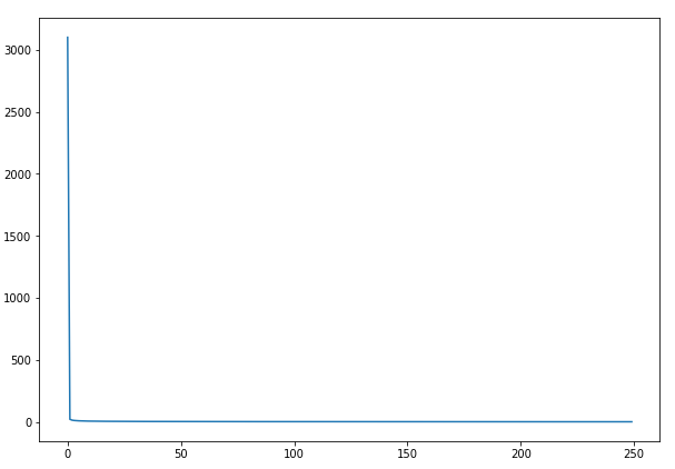
As you can see, not many epochs are needed to reach our final error cost.

Similarly, if you run the same script with sigmoid function at the output layer, the minimum error cost that you will achieve after 50000 epochs will be around 1.5 which is greater than 0.5, achieved with softmax.

Conclusion

Real-world neural networks are capable of solving multi-class classification problems. In this article, we saw how we can create a very simple neural network for multi-class classification, from scratch in Python. This is the final article of the series: "Neural Network from Scratch in Python". In the future articles, I will explain how we can create more specialized neural networks such as recurrent neural networks and convolutional neural networks from scratch in Python.