Dimensionality Reduction in Python with Scikit-Learn

Introduction

In machine learning, the performance of a model only benefits from more features up until a certain point. The more features are fed into a model, the more the dimensionality of the data increases. As the dimensionality increases, overfitting becomes more likely.

There are multiple techniques that can be used to fight overfitting, but dimensionality reduction is one of the most effective techniques. Dimensionality reduction selects the most important components of the feature space, preserving them and dropping the other components.

Why is Dimensionality Reduction Needed?

There are a few reasons that dimensionality reduction is used in machine learning: to combat computational cost, to control overfitting, and to visualize and help interpret high dimensional data sets.

Often in machine learning, the more features that are present in the dataset the better a classifier can learn. However, more features also means a higher computational cost. Not only can high dimensionality lead to long training times, more features often lead to an algorithm overfitting as it tries to create a model that explains all the features in the data.

Because dimensionality reduction reduces the overall number of features, it can reduce the computational demands associated with training a model but also helps combat overfitting by keeping the features that will be fed to the model fairly simple.

Dimensionality reduction can be used in both supervised and unsupervised learning contexts. In the case of unsupervised learning, dimensionality reduction is often used to preprocess the data by carrying out feature selection or feature extraction.

The primary algorithms used to carry out dimensionality reduction for unsupervised learning are Principal Component Analysis (PCA) and Singular Value Decomposition (SVD).

In the case of supervised learning, dimensionality reduction can be used to simplify the features fed into the machine learning classifier. The most common methods used to carry out dimensionality reduction for supervised learning problems is Linear Discriminant Analysis (LDA) and PCA, and it can be utilized to predict new cases.

Take note that the use cases described above are general use cases and not the only conditions these techniques are used in. After all, dimensionality reduction techniques are statistical methods and their use is not restricted by machine learning models.

Let's take some time to explain the ideas behind each of the most common dimensionality reduction techniques.

Principal Component Analysis

Principal Component Analysis (PCA) is a statistical method that creates new features or characteristics of data by analyzing the characteristics of the dataset. Essentially, the characteristics of the data are summarized or combined together. You can also conceive of Principal Component Analysis as "squishing" data down into just a few dimensions from much higher dimensions space.

To be more concrete, a drink might be described by many features, but many of these features will be redundant and relatively useless for identifying the drink in question. Rather than describing wine with features like aeration, C02 levels, etc., they could more easily be described by color, taste, and age.

Principal Component Analysis selects the "principal" or most influential characteristics of the dataset and creates features based on them. By choosing only the features with the most influence on the dataset, the dimensionality is reduced.

PCA preserves the correlations between variables when it creates new features. The principal components created by the technique are linear combinations of the original variables, calculated with concepts called eigenvectors.

It is assumed that the new components are orthogonal, or unrelated to one another.

PCA Implementation Example

Let's take a look at how PCA can be implemented in Scikit-Learn. We'll be using the Mushroom classification dataset for this.

First, we need to import all the modules we need, which includes PCA, train_test_split, and labeling and scaling tools:

import pandas as pd
import matplotlib.pyplot as plt
from sklearn.preprocessing import LabelEncoder, StandardScaler
from sklearn.decomposition import PCA
from sklearn.model_selection import train_test_split
import warnings
warnings.filterwarnings("ignore")

After we load in the data, we'll check for any null values. We'll also encode the data with the LabelEncoder. The class feature is the first column in the dataset, so we split up the features and labels accordingly:

m_data = pd.read_csv('mushrooms.csv')

# Machine learning systems work with integers, we need to encode these
# string characters into ints

encoder = LabelEncoder()

# Now apply the transformation to all the columns:
for col in m_data.columns:
    m_data[col] = encoder.fit_transform(m_data[col])

X_features = m_data.iloc[:,1:23]
y_label = m_data.iloc[:, 0]

We'll now scale the features with the standard scaler. This is optional as we aren't actually running the classifier, but it may impact how our data is analyzed by PCA:

# Scale the features
scaler = StandardScaler()
X_features = scaler.fit_transform(X_features)

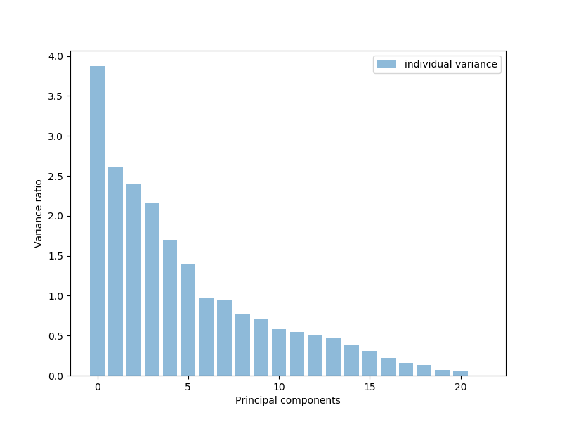
We'll now use PCA to get the list of features and plot which features have the most explanatory power, or have the most variance. These are the principle components. It looks like around 17 or 18 of the features explain the majority, almost 95% of our data:

# Visualize
pca = PCA()
pca.fit_transform(X_features)
pca_variance = pca.explained_variance_

plt.figure(figsize=(8, 6))
plt.bar(range(22), pca_variance, alpha=0.5, align='center', label='individual variance')
plt.legend()
plt.ylabel('Variance ratio')
plt.xlabel('Principal components')
plt.show()

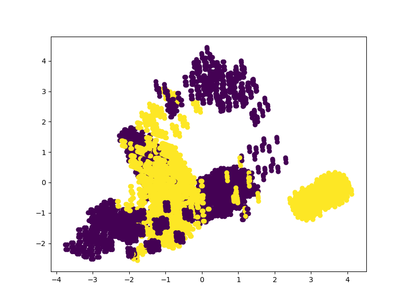
Let's convert the features into the 17 top features. We'll then plot a scatter plot of the data point classification based on these 17 features:

pca2 = PCA(n_components=17)
pca2.fit(X_features)
x_3d = pca2.transform(X_features)

plt.figure(figsize=(8,6))
plt.scatter(x_3d[:,0], x_3d[:,5], c=m_data['class'])
plt.show()

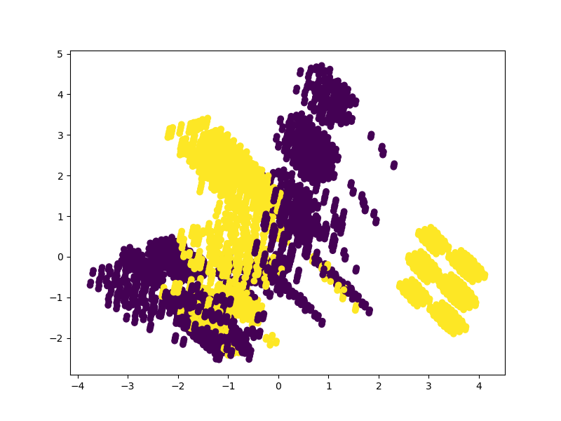
Let's also do this for the top 2 features and see how the classification changes:

pca3 = PCA(n_components=2)
pca3.fit(X_features)
x_3d = pca3.transform(X_features)

plt.figure(figsize=(8,6))
plt.scatter(x_3d[:,0], x_3d[:,1], c=m_data['class'])
plt.show()

Singular Value Decomposition

The purpose of Singular Value Decomposition is to simplify a matrix and make doing calculations with the matrix easier. The matrix is reduced to its constituent parts, similar to the goal of PCA. Understanding the ins and outs of SVD isn't completely necessary to implement it in your machine learning models, but having an intuition for how it works will give you a better idea of when to use it.

SVD can be carried out on either complex or real-valued matrices, but to make this explanation easier to understand, we'll go over the method of decomposing a real-valued matrix.

When doing SVD we have a matrix filled in with data and we want to reduce the number of columns the matrix has. This reduces the dimensionality of the matrix while still preserving as much of the variability in the data as possible.

We can say that Matrix A equals the transpose of matrix V:

$$
A = U * D * V^t
$$

Assuming we have some matrix A, we can represent that matrix as three other matrices called U, V, and D. Matrix A has the original x*y elements, while Matrix U is an orthogonal matrix containing x*x elements and Matrix V is a different orthogonal matrix containing y*y elements. Finally, D is a diagonal matrix containing x*y elements.

Decomposing values for a matrix involves converting the singular values in the original matrix into the diagonal values of the new matrix. Orthogonal matrices do not have their properties changed if they are multiplied by other numbers, and we can take advantage of this property to get an approximation of matrix A. When multiplying the orthogonal matrix together combined when the transpose of matrix V, we get a matrix that is equivalent to the original matrix A.

When we break/decompose matrix A down into U, D, and V, we then have three different matrices that contain the information of Matrix A.

It turns out that the left-most columns of the matrices hold the majority of our data, and we can select just these few columns to have a good approximation of Matrix A. This new matrix is much simpler and easier to work with, as it has far fewer dimensions.

SVD Implementation Example

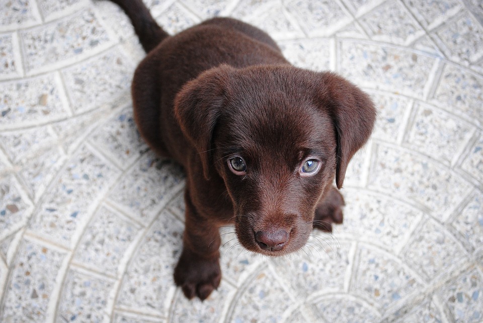
One of the most common ways that SVD is used is to compress images. After all, the pixel values that make up the red, green, and blue channels in the image can just be reduced and the result will be an image that is less complex but still contains the same image content. Let's try using SVD to compress an image and render it.

We'll use several functions to handle the compression of the image. We'll really only need Numpy and the Image function from the PIL library in order to accomplish this, since Numpy has a method to carry out the SVD calculation:

import numpy
from PIL import Image

First, we'll just write a function to load in the image and turn it into a Numpy array. We then want to select the red, green, and blue color channels from the image:

def load_image(image):
    image = Image.open(image)
    im_array = numpy.array(image)

    red = im_array[:, :, 0]
    green = im_array[:, :, 1]
    blue = im_array[:, :, 2]

    return red, green, blue

Now that we have the colors, we need to compress the color channels. We can start by calling Numpy's SVD function on the color channel we want. We'll then create an array of zeroes that we'll fill in after the matrix multiplication is completed. We then specify the singular value limit we want to use when doing the calculations:

def channel_compress(color_channel, singular_value_limit):
    u, s, v = numpy.linalg.svd(color_channel)
    compressed = numpy.zeros((color_channel.shape[0], color_channel.shape[1]))
    n = singular_value_limit

    left_matrix = numpy.matmul(u[:, 0:n], numpy.diag(s)[0:n, 0:n])
    inner_compressed = numpy.matmul(left_matrix, v[0:n, :])
    compressed = inner_compressed.astype('uint8')
    return compressed

red, green, blue = load_image("dog3.jpg")
singular_val_lim = 350

After this, we do matrix multiplication on the diagonal and the value limits in the U matrix, as described above. This gets us the left matrix and we then multiply it with the V matrix. This should get us the compressed values which we transform to the ‘uint8' type:

def compress_image(red, green, blue, singular_val_lim):
    compressed_red = channel_compress(red, singular_val_lim)
    compressed_green = channel_compress(green, singular_val_lim)
    compressed_blue = channel_compress(blue, singular_val_lim)

    im_red = Image.fromarray(compressed_red)
    im_blue = Image.fromarray(compressed_blue)
    im_green = Image.fromarray(compressed_green)

    new_image = Image.merge("RGB", (im_red, im_green, im_blue))
    new_image.show()
    new_image.save("dog3-edited.jpg")

compress_image(red, green, blue, singular_val_lim)

We'll be using this image of a dog to test our SVD compression on:

We also need to set the singular value limit we'll use, let's start with 600 for now:

red, green, blue = load_image("dog.jpg")
singular_val_lim = 350

Finally, we can get the compressed values for the three color channels and transform them from Numpy arrays into image components using PIL. We then just have to join the three channels together and show the image. This image should be a little smaller and simpler than the original image:

Indeed, if you inspect the size of the images, you'll notice that the compressed one is smaller, though we've also had a bit of lossy compression. You can see some noise in the image as well.

You can play around with adjusting the singular value limit. The lower the chosen limit the greater the compression will be, but at a certain point image artifact-ing will show up and the image will degrade in quality:

def compress_image(red, green, blue, singular_val_lim):
    compressed_red = channel_compress(red, singular_val_lim)
    compressed_green = channel_compress(green, singular_val_lim)
    compressed_blue = channel_compress(blue, singular_val_lim)

    im_red = Image.fromarray(compressed_red)
    im_blue = Image.fromarray(compressed_blue)
    im_green = Image.fromarray(compressed_green)

    new_image = Image.merge("RGB", (im_red, im_green, im_blue))
    new_image.show()

compress_image(red, green, blue, singular_val_lim)

Linear Discriminant Analysis

Linear Discriminant Analysis operates by projecting data from a multidimensional graph onto a linear graph. The easiest way to conceive of this is with a graph filled up with data points of two different classes. Assuming that there is no line that will neatly separate the data into two classes, the two dimensional graph can be reduced down into a 1D graph. This 1D graph can then be used to hopefully achieve the best possible separation of the data points.

When LDA is carried out there are two primary goals: minimizing the variance of the two classes and maximizing the distance between the means of the two data classes.

In order to achieve this, a new axis will be plotted in the 2D graph. This new axis should separate the two data points based on the previously mentioned criteria. Once the new axis has been created the data points within the 2D graph are redrawn along the new axis.

LDA carries out three different steps to move the original graph to the new axis. First, the separability between the classes has to be calculated, and this is based on the distance between the class means or the between-class variance. In the next step, the within class variance must be calculated, which is the distance between the mean and sample for the different classes. Finally, the lower dimensional space that maximizes the between class variance has to be constructed.

LDA works best when the means of the classes are far from each other. If the means of the distribution are shared it won't be possible for LDA to separate the classes with a new linear axis.

LDA Implementation Example

Finally, let's see how LDA can be used to carry out dimensionality reduction. Note that LDA can be used as a classification algorithm in addition to carrying out dimensionality reduction.

We'll be using the Titanic dataset for the following example.

Let's start off by making all our necessary imports:

import pandas as pd
import numpy as np
from sklearn.metrics import accuracy_score, f1_score
from sklearn.preprocessing import LabelEncoder, StandardScaler
from sklearn.discriminant_analysis import LinearDiscriminantAnalysis as LDA
from sklearn.model_selection import train_test_split
from sklearn.linear_model import LogisticRegression

We'll now load in our training data, which we'll divide into training and validation sets.

Though, we need to do a little data preprocessing first. Let's drop the Name, Cabin, and Ticket columns as they don't carry a lot of useful info. We also need to fill in any missing data, which we'll replace with median values in the case of the Age feature and an S in the case of the Embarked feature:

training_data = pd.read_csv("train.csv")

# Let's drop the cabin and ticket columns
training_data.drop(labels=['Cabin', 'Ticket'], axis=1, inplace=True)

training_data["Age"].fillna(training_data["Age"].median(), inplace=True)
training_data["Embarked"].fillna("S", inplace=True)

We also need to encode the non-numerical features. We'll encode both the Sex and Embarked columns. Let's drop the Name column as well, since it seems unlikely to be useful in classification:

encoder_1 = LabelEncoder()

# Fit the encoder on the data
encoder_1.fit(training_data["Sex"])

# Transform and replace the training data
training_sex_encoded = encoder_1.transform(training_data["Sex"])
training_data["Sex"] = training_sex_encoded

encoder_2 = LabelEncoder()
encoder_2.fit(training_data["Embarked"])

training_embarked_encoded = encoder_2.transform(training_data["Embarked"])
training_data["Embarked"] = training_embarked_encoded

# Assume the name is going to be useless and drop it
training_data.drop("Name", axis=1, inplace=True)

We need to scale the values, but the Scaler tool takes arrays, so the values we want to reshape need to be turned into arrays first. After that, we can scale the data:

# Remember that the scaler takes arrays
ages_train = np.array(training_data["Age"]).reshape(-1, 1)
fares_train = np.array(training_data["Fare"]).reshape(-1, 1)

scaler = StandardScaler()

training_data["Age"] = scaler.fit_transform(ages_train)
training_data["Fare"] = scaler.fit_transform(fares_train)

# Now to select our training and testing data
features = training_data.drop(labels=['PassengerId', 'Survived'], axis=1)
labels = training_data['Survived']

We can now select the training features and labels and use train_test_split to make our training and validation data. It's easy to do classification with LDA, you handle it just like you would any other classifier in Scikit-Learn.

Just fit the function on the training data and have it predict on the validation/testing data. We can then print metrics for the predictions against the actual values:

X_train, X_val, y_train, y_val = train_test_split(features, labels, test_size=0.2, random_state=27)

model = LDA()
model.fit(X_train, y_train)
preds = model.predict(X_val)
acc = accuracy_score(y_val, preds)
f1 = f1_score(y_val, preds)

print("Accuracy: {}".format(acc))
print("F1 Score: {}".format(f1))

Here's the print out:

Accuracy: 0.8100558659217877
F1 Score: 0.734375

When it comes to transforming the data and reducing dimensionality, let's run a Logistic Regression classifier on the data first so we can see what our performance is prior to dimensionality reduction:

logreg_clf = LogisticRegression()
logreg_clf.fit(X_train, y_train)
preds = logreg_clf.predict(X_val)
acc = accuracy_score(y_val, preds)
f1 = f1_score(y_val, preds)

print("Accuracy: {}".format(acc))
print("F1 Score: {}".format(f1))

Here's the results:

Accuracy: 0.8100558659217877
F1 Score: 0.734375

Now we will transform the data features by specifying a number of desired components for LDA and fitting the model on the features and labels. We then just transform the features and save it into a new variable. Let's print out the original and reduced number of features:

LDA_transform = LDA(n_components=1)
LDA_transform.fit(features, labels)
features_new = LDA_transform.transform(features)

# Print the number of features
print('Original feature #:', features.shape[1])
print('Reduced feature #:', features_new.shape[1])

# Print the ratio of explained variance
print(LDA_transform.explained_variance_ratio_)

Here's the print out for the above code:

Original feature #: 7
Reduced feature #: 1
[1.]

We now just have to do train/test split again with the new features and run the classifier again to see how performance changed:

X_train, X_val, y_train, y_val = train_test_split(features_new, labels, test_size=0.2, random_state=27)

logreg_clf = LogisticRegression()
logreg_clf.fit(X_train, y_train)
preds = logreg_clf.predict(X_val)
acc = accuracy_score(y_val, preds)
f1 = f1_score(y_val, preds)

print("Accuracy: {}".format(acc))
print("F1 Score: {}".format(f1))

Accuracy: 0.8212290502793296
F1 Score: 0.7500000000000001

Conclusion

We've gone over the major methods of dimensionality reduction techniques: Principal Component Analysis, Singular Value Decomposition, and Linear Discriminant Analysis. These are statistical techniques you can use to help your machine learning models perform better, combat overfitting, and assist in data analysis.

While these three techniques are the most commonly used dimensionality reduction techniques, others exist. Other dimensionality techniques include kernel approximation and isomap spectral embedding.