Random Projection: Theory and Implementation in Python with Scikit-Learn

Introduction

This guide is an in-depth introduction to an unsupervised dimensionality reduction technique called Random Projections. A Random Projection can be used to reduce the complexity and size of data, making the data easier to process and visualize. It is also a preprocessing technique for input preparation to a classifier or a regressor.

Random Projection is typically applied to highly-dimensional data, where other techniques such as Principal Component Analysis (PCA) can't do the data justice.

In this guide, we'll delve into the details of Johnson-Lindenstrauss lemma, which lays the mathematical foundation of Random Projections. We'll also show how to perform Random Projection using Python's Scikit-Learn library, and use it to transform input data to a lower-dimensional space.

Theory is theory, and practice is practice. As a practical illustration, we'll load the Reuters Corpus Volume I Dataset, and apply Gaussian Random Projection and Sparse Random Projection to it.

What is a Random Projection of a Dataset?

Put simply:

Random Projection is a method of dimensionality reduction and data visualization that simplifies the complexity of high-dimensional datasets.

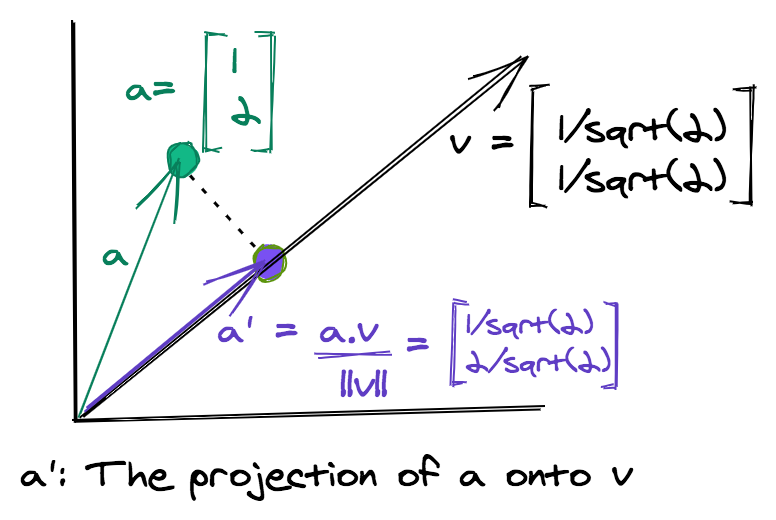
The method generates a new dataset by taking the projection of each data point along a randomly chosen set of directions. The projection of a single data point onto a vector is mathematically equivalent to taking the dot product of the point with the vector.

Given a data matrix \(X\) of dimensions \(mxn\) and a \(dxn\) matrix \(R\) whose columns are the vectors representing random directions, the Random Projection of \(X\) is given by \(X_p\).

$$X_p=XR$$

Each vector representing a random direction has dimensionality \(n\), which is the same as all data points of \(X\). If we take \(d\) random directions, then we end up with a \(d\) dimensional transformed dataset. For the purpose of this tutorial, we'll fix a few notations:

• m: Total example points/samples of input data.
• n: Total features/attributes of the input data. It is also the dimensionality of the original data.
• d: Dimensionality of the transformed data.

The idea of Random Projections is very similar to Principal Component Analysis (PCA), fundamentally. However, in PCA, the projection matrix is computed via eigenvectors, which can be computationally expensive for large matrices.

When performing Random Projection, the vectors are chosen randomly making it very efficient. The name "projection" may be a little misleading as the vectors are chosen randomly, the transformed points are mathematically not true projections but close to being true projections.

The data with reduced dimensions is easier to work with. Not only can it be visualized but it can also be used in the preprocessing stage to reduce the size of the original data.

A Simple Example

Just to understand how the transformation works, let's take the following simple example.

Suppose our input matrix \(X\) is given by:

$$X=\left[\begin{array}{cccc}1& 3& 2& 0\\ 0& 1& 2& 1\\ 1& 3& 0& 0\end{array}\right]$$

And the projection matrix is given by:

$$R=\frac{1}{2}\left[\begin{array}{cc}1& -1\\ 1& 1\\ 1& -1\\ 1& 1\end{array}\right]$$

The projection of X onto R is:

$$X_p=XR=\frac{1}{2}\left[\begin{array}{cc}6& 0\\ 4& 0\\ 4& 2\end{array}\right]$$

We started with three points in a four-dimensional space, and with clever matrix operations ended up with three transformed points in a two-dimensional space.

Note some important attributes of the projection matrix \(R\). Each column is a unit matrix, i.e., the norm of each column is one. Also, the dot product of all columns taken pairwise (in this case only column 1 and column 2) is zero, indicating that both column vectors are orthogonal to each other.

This makes the matrix, an Orthonormal Matrix. However, in the case of the Random Projection technique, the projection matrix does not have to be a true orthonormal matrix when very high-dimensional data is involved.

The success of Random Projection is based on an awesome mathematical finding known as Johnson-Lindenstrauss lemma, which is explained in detail in the following section!

The Johnson-Lindenstrauss lemma

The Johnson-Lindenstrauss lemma is the mathematical basis for Random Projection:

The Johnson-Lindenstrauss lemma states that if the data points lie in a very high-dimensional space, then projecting such points on simple random directions preserves their pairwise distances.

Preserving pairwise distances implies that the pairwise distances between points in the original space are the same or almost the same as the pairwise distance in the projected lower-dimensional space.

Thus, the structure of data and clusters within data are maintained in a lower-dimensional space, while the complexity and size of data are reduced substantially.

In this guide, we refer to the difference in the actual and projected pairwise distances as the "distortion" in data, which is introduced due to its projection in a new space.

Johnson-Lindenstrauss lemma also provides a "safe" measure of the number of dimensions to project the data points onto so that the error/distortion lies within a certain range, so finding the target number of dimensions is made easy.

Mathematically, given a pair of points \((x_1,x_2)\) and their corresponding projections \((x_1',x_2')\) defines an eps-embedding:

$$
(1 - \epsilon) |x_1 - x_2|^2 < |x_1' - x_2'|^2 < (1 + \epsilon) |x_1 - x_2|^2
$$

The Johnson-Lindenstrauss lemma specifies the minimum dimensions of the lower-dimensional space so that the above eps-embedding is maintained.

Determining the Random Directions of the Projection Matrix

Two well-known methods for determining the projection matrix are:

• Gaussian Random Projection: The projection matrix is constructed by choosing elements randomly from a Gaussian distribution with mean zero.

• Sparse Random Projection: This is a comparatively simpler method, where each vector component is a value from the set {-k,0,+k}, where k is a constant. One simple scheme for generating the elements of this matrix, also called the Achlioptas method is to set \(k=\sqrt 3\):

$$R_{ij}=\sqrt{3}\{\begin{array}{lll}+1& \text{ with probability }& \frac{1}{6}\\ 0& \text{ with probability }& \frac{2}{3}\\ -1& \text{ with probability }& \frac{1}{6}\end{array}$$

The method above is equivalent to choosing the numbers from {+k,0,-k} based on the outcome of the roll of a dice. If the dice score is 1, then choose +k. If the dice score is in the range [2,5], choose 0, and choose -k for a dice score of 6.

A more general method uses a density parameter to choose the Random Projection matrix. Setting \(s=\frac{1}{\text{density}}\), the elements of the Random Projection matrix are chosen as:

$$R_{ij}=\{\begin{array}{lll}+\sqrt{\frac{s}{d}}& \text{ with probability }& \frac{1}{2s}\\ 0& \text{ with probability }& 1-\frac{1}{s}\\ -\sqrt{\frac{s}{d}}& \text{ with probability }& \frac{1}{2s}\end{array}$$

The general recommendation is to set the density parameter to \(\frac{1}{\sqrt n}\).

As mentioned earlier, for both the Gaussian and sparse methods, the projection matrix is not a true orthonormal matrix. However, it has been shown that in high dimensional spaces, the randomly chosen matrix using either of the above two methods is close to an orthonormal matrix.

Random Projection Using Scikit-Learn

The Scikit-Learn library provides us with the random_projection module, that has three important classes/modules:

• johnson_lindenstrauss_min_dim(): For determining the minimum number of dimensions of transformed data when given a sample size m.
• GaussianRandomProjection: Performs Gaussian Random Projections.
• SparseRandomProjection: Performs Sparse Random Projections.

We'll demonstrate all the above three in the sections below, but first let's import the classes and functions we'll be using:

from sklearn.random_projection import SparseRandomProjection, johnson_lindenstrauss_min_dim
from sklearn.random_projection import GaussianRandomProjection
import numpy as np
from matplotlib import pyplot as plt
import sklearn.datasets as dt
from sklearn.metrics.pairwise import euclidean_distances

Determining the Minimum Number of Dimensions Via Johnson Lindenstrauss lemma

The johnson_lindenstrauss_min_dim() function determines the minimum number of dimensions d, which the input data can be mapped to when given the number of examples m, and the eps or \(\epsilon\) parameter.

The code below experiments with a different number of samples to determine the minimum size of the lower-dimensional space, which maintains a certain "safe" distortion of data.

Additionally, it plots log(d) against different values of eps for different sample sizes m.

An important thing to note is that the Johnson Lindenstrauss lemma determines the size of the lower-dimensional space \(d\) only based on the number of example points \(m\) in the input data. The number of attributes or features \(n\) of the original data is irrelevant:

eps = np.arange(0.001, 0.999, 0.01)
colors = ['b', 'g', 'm', 'c']
m = [1e1, 1e3, 1e7, 1e10]
for i in range(4):
    min_dim = johnson_lindenstrauss_min_dim(n_samples=m[i], eps=eps)
    label = 'Total samples = ' + str(m[i])
    plt.plot(eps, np.log10(min_dim), c=colors[i], label=label)
    
plt.xlabel('eps')
plt.ylabel('log$_{10}$(d)')
plt.axhline(y=3.5, color='k', linestyle=':')
plt.legend()
plt.show()

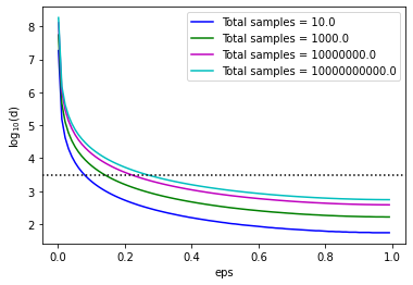
From the plot above, we can see that for small values of eps, d is quite large but decreases as eps approaches one. The dimensionality is below 3500 (the dotted black line) for mid to large values of eps.

This shows that applying Random Projections only makes sense to high-dimensional data, of the order of thousands of features. In such cases, a high reduction in dimensionality can be achieved.

Random Projections are, therefore, very successful for text or image data, which involve a large number of input features, where Principal Component Analysis would

Data Transformation

Python includes the implementation of both Gaussian Random Projections and Sparse Random Projections in its sklearn library via the two classes GaussianRandomProjection and SparseRandomProjection respectively. Some important attributes for these classes are (the list is not exhaustive):

• n_components: Number of dimensions of the transformed data. If it is set to auto, then the optimal dimensions are determined before projection
• eps: The parameter of Johnson-Lindenstrauss lemma, which controls the number of dimensions so that the distortion in projected data is kept within a certain bound.
• density: Only applicable for SparseRandomProjection. The default value is auto, which sets \(s=\frac{1}{\sqrt n}\) for the selection of the projection matrix.

Like other dimensionality reduction classes of sklearn, both these classes include the standard fit() and fit_transform() methods. A notable set of attributes, which come in handy are:

• n_components: The number of dimensions of the new space on which the data is projected.
• components_: The transformation or projection matrix.
• density_: Only applicable to SparseRandomProjection. It is the value of density based on which the elements of the projection matrix are computed.

Random Projection with GaussianRandomProjection

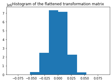
Let's start off with the GaussianRandomProjection class. The values of the projection matrix are plotted as a histogram and we can see that they follow a Gaussian distribution with mean zero. The size of the data matrix is reduced from 5000 to 3947:

X_rand = np.random.RandomState(0).rand(100, 5000)
proj_gauss = GaussianRandomProjection(random_state=0)
X_transformed = proj_gauss.fit_transform(X_rand)

# Print the size of the transformed data
print('Shape of transformed data: ' + str(X_transformed.shape))

# Generate a histogram of the elements of the transformation matrix
plt.hist(proj_gauss.components_.flatten())
plt.title('Histogram of the flattened transformation matrix')
plt.show()

This code results in:

Shape of transformed data: (100, 3947)

Random Projection with SparseRandomProjection

The code below demonstrates how data transformation can be made using a Sparse Random Projection. The entire transformation matrix is composed of three distinct values, whose frequency plot is also shown below.

Note that the transformation matrix is a SciPy sparse csr_matrix. The following code accesses the non-zero values of the csr_matrix and stores them in p. Next, it uses p to get the counts of the elements of the sparse projection matrix:

proj_sparse = SparseRandomProjection(random_state=0)
X_transformed = proj_sparse.fit_transform(X_rand)

# Print the size of the transformed data
print('Shape of transformed data: ' + str(X_transformed.shape))

# Get data of the transformation matrix and store in p. 
# p consists of only 2 non-zero distinct values, i.e., pos and neg
# pos and neg are determined below
p = proj_sparse.components_.data
total_elements = proj_sparse.components_.shape[0] *\
                  proj_sparse.components_.shape[1]
pos = p[p>0][0]
neg = p[p<0][0]
print('Shape of transformation matrix: '+ str(proj_sparse.components_.shape))
counts = (sum(p==neg), total_elements - len(p), sum(p==pos))
# Histogram of the elements of the transformation matrix
plt.bar([neg, 0, pos], counts, width=0.1)
plt.xticks([neg, 0, pos])
plt.suptitle('Histogram of flattened transformation matrix, ' + 
             'density = ' +
             '{:.2f}'.format(proj_sparse.density_))
plt.show()

This results in:

Shape of transformed data: (100, 3947)
Shape of transformation matrix: (3947, 5000)

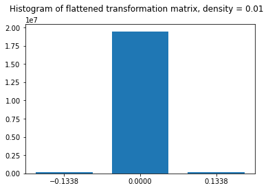
The histogram is in agreement with the method of generating a sparse Random Projection matrix as discussed in the previous section. The zero is selected with probability (1-1/100 = 0.99), hence around 99% of values of this matrix are zero. Utilizing the data structures and routines for sparse matrices makes this transformation method very fast and efficient on large datasets.

Practical Random Projections With the Reuters Corpus Volume 1 Dataset

This section illustrates Random Projections on the Reuters Corpus Volume I Dataset. The dataset is freely accessible online, though for our purposes, it's easiest to load via Scikit-Learn.

The sklearn.datasets module contains a fetch_rcv1() function that downloads and imports the dataset.

The RCV1 dataset is a multi-label dataset, i.e., each data point can belong to multiple classes at the same time, and consists of 103 classes. Each data point has a dimensionality of a whopping 47,236, making it an ideal case for applying fast and cheap Random Projections.

To demonstrate the effectiveness of Random Projections, and to keep things simple, we'll select 500 data points that belong to at least one of the first three classes. The fetch_rcv1() function retrieves the dataset and returns an object with data and targets, both of which are sparse CSR matrices from SciPy.

Let's fetch the Reuters Corpus and prepare it for data transformation:

total_points = 500
# Fetch the dataset
dat = dt.fetch_rcv1()
# Select the sparse matrix's non-zero targets
target_nz = dat.target.nonzero()
# Select only indices of target_nz for data points that belong to 
# either of class 1,2,3
ind_class_123 = np.asarray(np.where((target_nz[1]==0) |\
                                    (target_nz[1]==1) |\
                                    (target_nz[1] == 2))).flatten()
# Choose only 500 indices randomly
np.random.seed(0)
ind_class_123 = np.random.choice(ind_class_123, total_points, 
                                 replace=False)

# Retrieve the row indices of data matrix and target matrix
row_ind = target_nz[0][ind_class_123]
X = dat.data[row_ind,:]
y = np.array(dat.target[row_ind,0:3].todense())

After data preparation, we need a function that creates a visualization of the projected data. To have an idea of the quality of transformation, we can compute the following three matrices:

• dist_raw: Matrix of the pairwise Euclidean distances of the actual data points.
• dist_transform: Matrix of the pairwise Euclidean distances of the transformed data points.
• abs_diff: Matrix of the absolute difference of dist_raw and dist_actual

The abs_diff_dist matrix is a good indicator of the quality of the data transformation. Close to zero or small values in this matrix indicate low distortion and a good transformation. We can directly display an image of this matrix or generate a histogram of its values to visually assess the transformation. We can also compute the average of all the values of this matrix to get a single quantitative measure for comparison.

The function create_visualization() creates three plots. The first graph is a scatter plot of projected points along the first two random directions. The second plot is an image of the absolute difference matrix and the third is the histogram of the values of the absolute difference matrix:

def create_visualization(X_transform, y, abs_diff):
    fig,ax = plt.subplots(nrows=1, ncols=3, figsize=(20,7))

    plt.subplot(131)
    plt.scatter(X_transform[y[:,0]==1,0], X_transform[y[:,0]==1,1], c='r', alpha=0.4)
    plt.scatter(X_transform[y[:,1]==1,0], X_transform[y[:,1]==1,1], c='b', alpha=0.4)
    plt.scatter(X_transform[y[:,2]==1,0], X_transform[y[:,2]==1,1], c='g', alpha=0.4)
    plt.legend(['Class 1', 'Class 2', 'Class 3'])
    plt.title('Projected data along first two dimensions')

    plt.subplot(132)
    plt.imshow(abs_diff)
    plt.colorbar()
    plt.title('Visualization of absolute differences')

    plt.subplot(133)
    ax = plt.hist(abs_diff.flatten())
    plt.title('Histogram of absolute differences')

    fig.subplots_adjust(wspace=.3) 

Reuters Dataset: Gaussian Random Projection

Let's apply Gaussian Random Projection to the Reuters dataset. The code below runs a for loop for different eps values. If the minimum safe dimensions returned by johnson_lindenstrauss_min_dim is less than the actual data dimensions, then it calls the fit_transform() method of GaussianRandomProjection. The create_visualization() function is then called to create a visualization for that value of eps.

At every iteration, the code also stores the mean absolute difference and the percentage reduction in dimensionality achieved by Gaussian Random Projection:

reduction_dim_gauss = []
eps_arr_gauss = []
mean_abs_diff_gauss = []
for eps in np.arange(0.1, 0.999, 0.2):

    min_dim = johnson_lindenstrauss_min_dim(n_samples=total_points, eps=eps)
    if min_dim > X.shape[1]:
        continue
    gauss_proj = GaussianRandomProjection(random_state=0, eps=eps)
    X_transform = gauss_proj.fit_transform(X)
    dist_raw = euclidean_distances(X)
    dist_transform = euclidean_distances(X_transform)
    abs_diff_gauss = abs(dist_raw - dist_transform) 

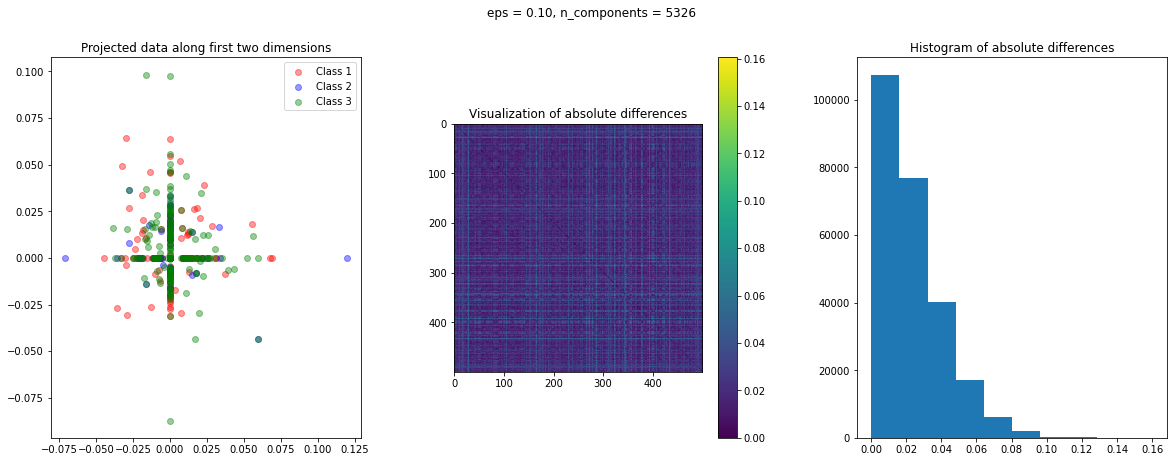
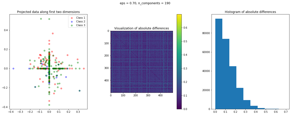
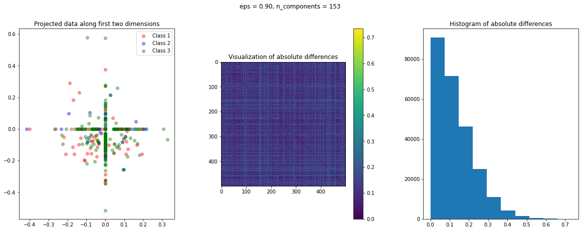
    create_visualization(X_transform, y, abs_diff_gauss)
    plt.suptitle('eps = ' + '{:.2f}'.format(eps) + ', n_components = ' + str(X_transform.shape[1]))
    
    reduction_dim_gauss.append(100-X_transform.shape[1]/X.shape[1]*100)
    eps_arr_gauss.append(eps)
    mean_abs_diff_gauss.append(np.mean(abs_diff_gauss.flatten()))

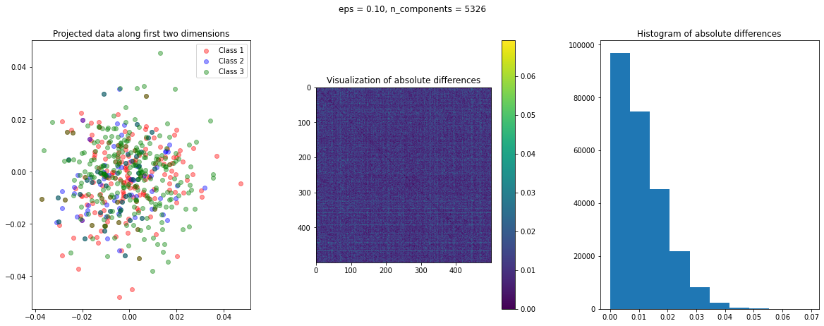
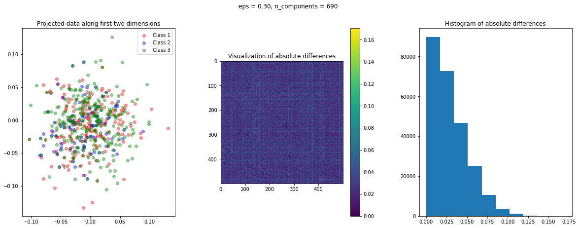
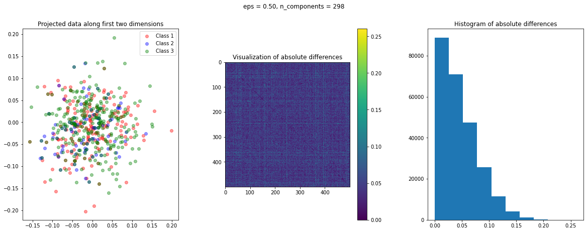
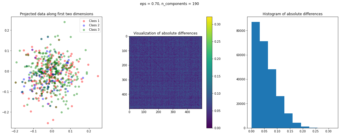
The images of the absolute difference matrix and its corresponding histogram indicate that most of the values are close to zero. Hence, a large majority of the pair of points maintain their actual distance in the low dimensional space, retaining the original structure of data.

To assess the quality of transformation, let's plot the mean absolute difference against eps. Also, the higher the value of eps, the greater the dimensionality reduction. Let's also plot the percentage reduction vs. eps in a second sub-plot:

fig,ax = plt.subplots(nrows=1, ncols=2, figsize=(10,5))
plt.subplot(121)
plt.plot(eps_arr_gauss, mean_abs_diff_gauss, marker='o', c='g')
plt.xlabel('eps')
plt.ylabel('Mean absolute difference')

plt.subplot(122)
plt.plot(eps_arr_gauss, reduction_dim_gauss, marker = 'o', c='m')
plt.xlabel('eps')
plt.ylabel('Percentage reduction in dimensionality')

fig.subplots_adjust(wspace=.4) 
plt.suptitle('Assessing the Quality of Gaussian Random Projections')
plt.show()

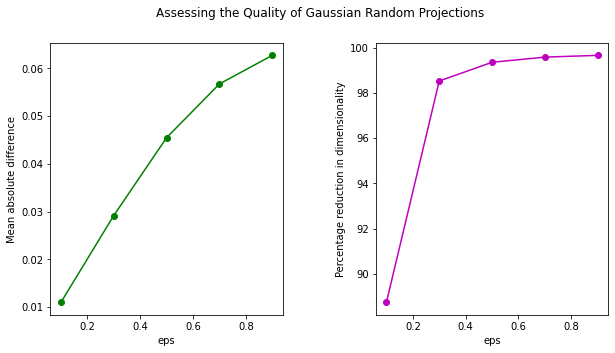
We can see that using Gaussian Random Projection we can reduce the dimensionality of data to more than 99%! Though, this does come at the cost of a higher distortion of data.

Reuters Dataset: Sparse Random Projection

We can do a similar comparison with sparse Random Projection:

reduction_dim_sparse = []
eps_arr_sparse = []
mean_abs_diff_sparse = []
for eps in np.arange(0.1, 0.999, 0.2):

    min_dim = johnson_lindenstrauss_min_dim(n_samples=total_points, eps=eps)
    if min_dim > X.shape[1]:
        continue
    sparse_proj = SparseRandomProjection(random_state=0, eps=eps, dense_output=1)
    X_transform = sparse_proj.fit_transform(X)
    dist_raw = euclidean_distances(X)
    dist_transform = euclidean_distances(X_transform)
    abs_diff_sparse = abs(dist_raw - dist_transform) 

    create_visualization(X_transform, y, abs_diff_sparse)
    plt.suptitle('eps = ' + '{:.2f}'.format(eps) + ', n_components = ' + str(X_transform.shape[1]))
    
    reduction_dim_sparse.append(100-X_transform.shape[1]/X.shape[1]*100)
    eps_arr_sparse.append(eps)
    mean_abs_diff_sparse.append(np.mean(abs_diff_sparse.flatten()))

In the case of Random Projection, the absolute difference matrix appears similar to the one of Gaussian projection. The projected data on the first two dimensions, however, has a more interesting pattern, with many points mapped on the coordinate axis.

Let's also plot the mean absolute difference and percentage reduction in dimensionality for various values of the eps parameter:

fig,ax = plt.subplots(nrows=1, ncols=2, figsize=(10,5))
plt.subplot(121)
plt.plot(eps_arr_sparse, mean_abs_diff_sparse, marker='o', c='g')
plt.xlabel('eps')
plt.ylabel('Mean absolute difference')

plt.subplot(122)
plt.plot(eps_arr_sparse, reduction_dim_sparse, marker = 'o', c='m')
plt.xlabel('eps')
plt.ylabel('Percentage reduction in dimensionality')

fig.subplots_adjust(wspace=.4) 
plt.suptitle('Assessing the Quality of Sparse Random Projections')
plt.show()

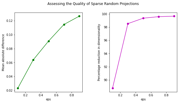
The trend of the two graphs is similar to that of a Gaussian Projection. However, the mean absolute difference for Gaussian Projection is lower than that of Random Projection.

Conclusions

In this guide, we discussed the details of two main types of Random Projections, i.e., Gaussian and sparse Random Projection.

We presented the details of the Johnson-Lindenstrauss lemma, the mathematical basis for these methods. We then showed how this method can be used to transform data using Python's sklearn library.

We also illustrated the two methods on a real-life Reuters Corpus Volume I Dataset.

We encourage the reader to try out this method in supervised classification or regression tasks at the preprocessing stage when dealing with very high-dimensional datasets.