
Introduction
Ensemble classification models can be powerful machine learning tools capable of achieving excellent performance and generalizing well to new, unseen datasets.
The value of an ensemble classifier is that, in joining together the predictions of multiple classifiers, it can correct for errors made by any individual classifier, leading to better accuracy overall. Let's take a look at the different ensemble classification methods and see how these classifiers can be implemented in Scikit-Learn.
What are Ensemble Models in Machine Learning?

Credit: Pixabay
Ensemble models are an ensemble learning method that combines different algorithms together. In this sense, it is a meta-algorithm rather than an algorithm itself. Ensemble learning methods are valuable because they can improve the performance of a predictive model.
Ensemble learning methods work off of the idea that tying the predictions of multiple classifiers together will lead to better performance by either improving prediction accuracy or reducing aspects like bias and variance.
In general, an ensemble model falls into one of two categories: sequential approaches and parallel approaches.
A sequential ensemble model operates by having the base learners/models generated in sequence. Sequential ensemble methods are typically used to try and increase overall performance, as the ensemble model can compensate for inaccurate predictions by re-weighting the examples that were previously misclassified. A notable example of this is AdaBoost.
A parallel model is, as you may be able to guess, methods that rely on creating and training the base learners in parallel. Parallel methods aim to reduce the error rate by training many models in parallel and averaging the results together. A notable example of a parallel method is the Random Forest Classifier.
Another way of thinking about this is a distinction between homogenous and heterogeneous learners. While most of the ensemble learning methods use homogeneous base learners (many of the same type of learners), some ensemble methods use heterogeneous learners (different learning algorithms joined together).
To recap:
- Sequential models try to increase performance by re-weighting examples, and models are generated in sequence.
- Parallel models work by averaging results together after training many models at the same time.
We'll now cover different methods of employing these models to solve machine learning classification problems.
Different Ensemble Classification Methods
Bagging
Credit: Wikimedia Commons
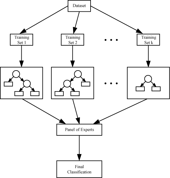
Bagging, also known as bootstrap aggregating, is a classification method that aims to reduce the variance of estimates by averaging multiple estimates together. Bagging creates subsets from the main dataset that the learners are trained on.
In order for the predictions of the different classifiers to be aggregated, either an averaging is used for regression, or a voting approach is used for classification (based on the decision of the majority).
One example of a bagging classification method is the Random Forests Classifier. In the case of the random forests classifier, all the individual trees are trained on a different sample of the dataset.
The tree is also trained using random selections of features. When the results are averaged together, the overall variance decreases and the model performs better as a result.
Boosting
Boosting algorithms are capable of taking weak, underperforming models and converting them into strong models. The idea behind boosting algorithms is that you assign many weak learning models to the datasets, and then the weights for misclassified examples are tweaked during subsequent rounds of learning.
The predictions of the classifiers are aggregated and then the final predictions are made through a weighted sum (in the case of regressions), or a weighted majority vote (in the case of classification).
AdaBoost is one example of a boosting classifier method, as is Gradient Boosting, which was derived from the aforementioned algorithm.
If you'd like to read more about Gradient Boosting and the theory behind it, we've already covered that in a previous article.
Stacking
Credit: Wikimedia Commons
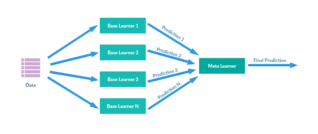
Stacking algorithms are an ensemble learning method that combines the decision of different regression or classification algorithms. The component models are trained on the entire training dataset. After these component models are trained, a meta-model is assembled from the different models and then it's trained on the outputs of the component models. This approach typically creates a heterogeneous ensemble because the component models are usually different algorithms.
Example Implementations
Now that we've explored different methods we can use to create ensemble models, let's take a look at how we could implement a classifier using the different methods.
Though, before we can take a look at different ways of implementing ensemble classifiers, we need to select a dataset to use and do some preprocessing of the dataset.
We'll be using the Titanic dataset, which can be downloaded here. Let's do some preprocessing of the data in order to get rid of missing values and scale the data to a uniform range. Then we can go about setting up the ensemble classifiers.
Data Preprocessing
To begin with, we'll start by importing all functions we need from their respective libraries. We'll be using Pandas and Numpy to load and transform the data, as well as the LabelEncoder and StandardScaler tools.
We'll also need the machine learning metrics and the train_test_split function. Finally, we'll need the classifiers we want to use:
import pandas as pd
import numpy as np
import warnings

from sklearn.preprocessing import LabelEncoder, StandardScaler
from sklearn.metrics import accuracy_score, f1_score, log_loss
from sklearn.model_selection import train_test_split, KFold, cross_val_score

from sklearn.svm import SVC
from sklearn.linear_model import LogisticRegression
from sklearn.tree import DecisionTreeClassifier
from sklearn.ensemble import VotingClassifier
from sklearn.ensemble import BaggingClassifier
from sklearn.ensemble import AdaBoostClassifier, RandomForestClassifier, ExtraTreesClassifier
We'll start by loading in the training and testing data and then creating a function to check for the presence of any null values:
training_data = pd.read_csv("train.csv")
testing_data = pd.read_csv("test.csv")

def get_nulls(training, testing):
    print("Training Data:")
    print(pd.isnull(training).sum())
    print("Testing Data:")
    print(pd.isnull(testing).sum())

get_nulls(training_data, testing_data)
Check out our hands-on, practical guide to learning Git, with best-practices, industry-accepted standards, and included cheat sheet. Stop Googling Git commands and actually learn it!
As it happens, there are a lot of missing values in the Age and Cabin categories.
Training Data:
PassengerId      0
Survived         0
Pclass           0
Name             0
Sex              0
Age            177
SibSp            0
Parch            0
Ticket           0
Fare             0
Cabin          687
Embarked         2
dtype: int64
Testing Data:
PassengerId      0
Pclass           0
Name             0
Sex              0
Age             86
SibSp            0
Parch            0
Ticket           0
Fare             1
Cabin          327
Embarked         0
dtype: int64
We're going to start by dropping some of the columns that will likely be useless - the Cabin column and the Ticket column. The Cabin column has far too many missing values and the Ticket column is simply comprised of too many categories to be useful.
After that we will need to impute some missing values. When we do so, we must account for how the dataset is slightly right skewed (young ages are slightly more prominent than older ages). We'll use the median values when we impute the data because due to large outliers taking the average values would give us imputed values that are far from the center of the dataset:
# Drop the cabin column, as there are too many missing values
# Drop the ticket numbers too, as there are too many categories
# Drop names as they won't really help predict survivors

training_data.drop(labels=['Cabin', 'Ticket', 'Name'], axis=1, inplace=True)
testing_data.drop(labels=['Cabin', 'Ticket', 'Name'], axis=1, inplace=True)

# Taking the mean/average value would be impacted by the skew
# so we should use the median value to impute missing values

training_data["Age"].fillna(training_data["Age"].median(), inplace=True)
testing_data["Age"].fillna(testing_data["Age"].median(), inplace=True)
training_data["Embarked"].fillna("S", inplace=True)
testing_data["Fare"].fillna(testing_data["Fare"].median(), inplace=True)

get_nulls(training_data, testing_data)
Now we can see there's no more missing values:
Training Data:
PassengerId    0
Survived       0
Pclass         0
Name           0
Sex            0
Age            0
SibSp          0
Parch          0
Fare           0
Embarked       0
dtype: int64
Testing Data:
PassengerId    0
Pclass         0
Name           0
Sex            0
Age            0
SibSp          0
Parch          0
Fare           0
Embarked       0
dtype: int64
We're now going to need to encode the non-numerical data. Let's set up a LabelEncoder and fit it on the Sex feature and then transform the data with the encoder. We'll then replace the values in the Sex feature with those that have been encoded and then do the same for the Embarked feature.
Finally, let's scale the data using the StandardScaler, so there aren't huge fluctuations in values.
encoder_1 = LabelEncoder()
# Fit the encoder on the data
encoder_1.fit(training_data["Sex"])

# Transform and replace training data
training_sex_encoded = encoder_1.transform(training_data["Sex"])
training_data["Sex"] = training_sex_encoded
test_sex_encoded = encoder_1.transform(testing_data["Sex"])
testing_data["Sex"] = test_sex_encoded

encoder_2 = LabelEncoder()
encoder_2.fit(training_data["Embarked"])

training_embarked_encoded = encoder_2.transform(training_data["Embarked"])
training_data["Embarked"] = training_embarked_encoded
testing_embarked_encoded = encoder_2.transform(testing_data["Embarked"])
testing_data["Embarked"] = testing_embarked_encoded

# Any value we want to reshape needs be turned into array first
ages_train = np.array(training_data["Age"]).reshape(-1, 1)
fares_train = np.array(training_data["Fare"]).reshape(-1, 1)
ages_test = np.array(testing_data["Age"]).reshape(-1, 1)
fares_test = np.array(testing_data["Fare"]).reshape(-1, 1)

# Scaler takes arrays
scaler = StandardScaler()

training_data["Age"] = scaler.fit_transform(ages_train)
training_data["Fare"] = scaler.fit_transform(fares_train)
testing_data["Age"] = scaler.fit_transform(ages_test)
testing_data["Fare"] = scaler.fit_transform(fares_test)
Now that our data has been preprocessed, we can select our features and labels and then use the train_test_split function to divide our entire training data up into training and testing sets:
# Now to select our training/testing data
X_features = training_data.drop(labels=['PassengerId', 'Survived'], axis=1)
y_labels = training_data['Survived']

print(X_features.head(5))

# Make the train/test data from validation

X_train, X_val, y_train, y_val = train_test_split(X_features, y_labels, test_size=0.1, random_state=27)
We're now ready to start implementing ensemble classification methods.
Simple Averaging Approach
Before we get into the big three ensemble methods we covered earlier, let's cover a very quick and easy method of using an ensemble approach - averaging predictions. We simply add the different predicted values of our chosen classifiers together and then divide by the total number of classifiers, using floor division to get a whole value.
In this test case we'll be using logistic regression, a Decision Tree Classifier, and the Support Vector Classifier. We fit the classifiers on the data and then save the predictions as variables. Then we simply add the predictions together and divide:
LogReg_clf = LogisticRegression()
DTree_clf = DecisionTreeClassifier()
SVC_clf = SVC()

LogReg_clf.fit(X_train, y_train)
DTree_clf.fit(X_train, y_train)
SVC_clf.fit(X_train, y_train)

LogReg_pred = LogReg_clf.predict(X_val)
DTree_pred = DTree_clf.predict(X_val)
SVC_pred = SVC_clf.predict(X_val)

averaged_preds = (LogReg_pred + DTree_pred + SVC_pred)//3
acc = accuracy_score(y_val, averaged_preds)
print(acc)
Here's the accuracy we got from this method:
0.8444444444444444
Voting\Stacking Classification Example
When it comes to creating a stacking/voting classifier, Scikit-Learn provides us with some handy functions that we can use to accomplish this.
The VotingClassifier takes in a list of different estimators as arguments and a voting method. The hard voting method uses the predicted labels and a majority rules system, while the soft voting method predicts a label based on the argmax/largest predicted value of the sum of the predicted probabilities.
After we provide the desired classifiers, we need to fit the resulting ensemble classifier object. We can then get predictions and use accuracy metrics:
voting_clf = VotingClassifier(estimators=[('SVC', SVC_clf), ('DTree', DTree_clf), ('LogReg', LogReg_clf)], voting='hard')
voting_clf.fit(X_train, y_train)
preds = voting_clf.predict(X_val)
acc = accuracy_score(y_val, preds)
l_loss = log_loss(y_val, preds)
f1 = f1_score(y_val, preds)

print("Accuracy is: " + str(acc))
print("Log Loss is: " + str(l_loss))
print("F1 Score is: " + str(f1))
Here's what the metrics have to say about the VotingClassifier's performance:
Accuracy is: 0.8888888888888888
Log Loss is: 3.8376684749044165
F1 Score is: 0.8484848484848486
Bagging Classification Example
Here's how we can implement bagging classification with Scikit-Learn. Sklearn's BaggingClassifier takes in a chosen classification model as well as the number of estimators that you want to use - you can use a model like Logistic Regression or Decision Trees.
Sklearn also provides access to the RandomForestClassifier and the ExtraTreesClassifier, which are modifications of the decision tree classification. These classifiers can also be used alongside the K-folds cross-validation tool.
We'll compare several different bagging classification approaches here, printing out the mean results of the K-fold cross validation score:
logreg_bagging_model = BaggingClassifier(base_estimator=LogReg_clf, n_estimators=50, random_state=12)
dtree_bagging_model = BaggingClassifier(base_estimator=DTree_clf, n_estimators=50, random_state=12)
random_forest = RandomForestClassifier(n_estimators=100, random_state=12)
extra_trees = ExtraTreesClassifier(n_estimators=100, random_state=12)

def bagging_ensemble(model):
    k_folds = KFold(n_splits=20, random_state=12)
    results = cross_val_score(model, X_train, y_train, cv=k_folds)
    print(results.mean())

bagging_ensemble(logreg_bagging_model)
bagging_ensemble(dtree_bagging_model)
bagging_ensemble(random_forest)
bagging_ensemble(extra_trees)
Here's the results we got from the classifiers:
0.7865853658536585
0.8102439024390244
0.8002439024390245
0.7902439024390244
Boosting Classification Example
Finally, we'll take a look at how to use a boosting classification method. As mentioned, there's a separate article on the topic of Gradient Boosting you can read here.
Scikit-Learn has a built-in AdaBoost classifier, which takes in a given number of estimators as the first argument. We can try using a for loop to see how the classification performance changes at different values, and we can also combine it with the K-Folds cross validation tool:
k_folds = KFold(n_splits=20, random_state=12)

num_estimators = [20, 40, 60, 80, 100]

for i in num_estimators:
    ada_boost = AdaBoostClassifier(n_estimators=i, random_state=12)
    results = cross_val_score(ada_boost, X_train, y_train, cv=k_folds)
    print("Results for {} estimators:".format(i))
    print(results.mean())
Here's the results we got:
Results for 20 estimators:
0.8015243902439024
Results for 40 estimators:
0.8052743902439025
Results for 60 estimators:
0.8053048780487805
Results for 80 estimators:
0.8040243902439024
Results for 100 estimators:
0.8027743902439024
Summing Up
We've covered the ideas behind three different ensemble classification techniques: voting\stacking, bagging, and boosting.
Scikit-Learn allows you to easily create instances of the different ensemble classifiers. These ensemble objects can be combined with other Scikit-Learn tools like K-Folds cross validation.

