
Introduction
In this tutorial, we'll discuss the details of generating different synthetic datasets using the Numpy and Scikit-learn libraries. We'll see how different samples can be generated from various distributions with known parameters.
We'll also discuss generating datasets for different purposes, such as regression, classification, and clustering. At the end we'll see how we can generate a dataset that mimics the distribution of an existing dataset.
The Need for Synthetic Data
In data science, synthetic data plays a very important role. It allows us to test a new algorithm under controlled conditions. In other words, we can generate data that tests a very specific property or behavior of our algorithm.
For example, we can test its performance on balanced vs. imbalanced datasets, or we can evaluate its performance under different noise levels. By doing this, we can establish a baseline of our algorithm's performance under various scenarios.
There are many other instances, where synthetic data may be needed. For example, real data may be hard or expensive to acquire, or it may have too few data-points. Another reason is privacy, where real data cannot be revealed to others.
Setting Up
Before we write code for synthetic data generation, let's import the required libraries:
import numpy as np

# Needed for plotting
import matplotlib.colors
import matplotlib.pyplot as plt
from mpl_toolkits.mplot3d import Axes3D

# Needed for generating classification, regression and clustering datasets
import sklearn.datasets as dt

# Needed for generating data from an existing dataset
from sklearn.neighbors import KernelDensity
from sklearn.model_selection import GridSearchCV
Then, we'll have some useful variables in the beginning:
# Define the seed so that results can be reproduced
seed = 11
rand_state = 11

# Define the color maps for plots
color_map = plt.cm.get_cmap('RdYlBu')
color_map_discrete = matplotlib.colors.LinearSegmentedColormap.from_list("", ["red","cyan","magenta","blue"])
Generating 1D Samples from Known Distributions
Now, we'll talk about generating sample points from known distributions in 1D.
The random module from numpy offers a wide range of ways to generate random numbers sampled from a known distribution with a fixed set of parameters. For reproduction purposes, we'll pass the seed to the RandomState call and as long as we use that same seed, we'll get the same numbers.
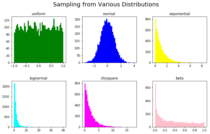
Let's define a distribution list, such as uniform, normal, exponential, etc, a parameter list, and a color list so that we can visually discern between these:
rand = np.random.RandomState(seed)

dist_list = ['uniform','normal','exponential','lognormal','chisquare','beta']
param_list = ['-1,1','0,1','1','0,1','2','0.5,0.9']
colors_list = ['green','blue','yellow','cyan','magenta','pink']
Now, we'll pack these into subplots of a Figure for visualization and generate synthetic data based on these distributions, parameters and assign them adequate colors.
This is done via the eval() function, which we use to generate a Python expression. For example, we can use rand.exponential(1, 5000) to generate samples from an exponential distribution of scale 1 and the size of 5000.
Here, we'll use our dist_list, param_list and color_list to generate these calls:
fig,ax = plt.subplots(nrows=2, ncols=3,figsize=(12,7))
plt_ind_list = np.arange(6)+231

for dist, plt_ind, param, colors in zip(dist_list, plt_ind_list, param_list, colors_list):
    x = eval('rand.'+dist+'('+param+',5000)')

    plt.subplot(plt_ind)
    plt.hist(x,bins=50,color=colors)
    plt.title(dist)

fig.subplots_adjust(hspace=0.4,wspace=.3)
plt.suptitle('Sampling from Various Distributions',fontsize=20)
plt.show()
This results in:
Synthetic Data for Regression
The sklearn.datasets package has functions for generating synthetic datasets for regression. Here, we discuss linear and non-linear data for regression.
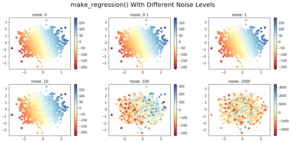
The make_regression() function returns a set of input data points (regressors) along with their output (target). This function can be adjusted with the following parameters:
n_features- number of dimensions/features of the generated datanoise- standard deviation of gaussian noisen_samples- number of samples
The response variable is a linear combination of the generated input set.
A response variable is something that's dependent on other variables, in this particular case, a target feature that we're trying to predict using all the other input features.
In the code below, synthetic data has been generated for different noise levels and consists of two input features and one target variable. The changing color of the input points shows the variation in the target's value, corresponding to the data point. The data is generated in 2D for better visualization, but high-dimensional data can be created using the n_features parameter:
map_colors = plt.cm.get_cmap('RdYlBu')
fig,ax = plt.subplots(nrows=2, ncols=3,figsize=(16,7))
plt_ind_list = np.arange(6)+231

for noise,plt_ind in zip([0,0.1,1,10,100,1000],plt_ind_list):
    x,y = dt.make_regression(n_samples=1000,
                             n_features=2,
                             noise=noise,
                             random_state=rand_state)

    plt.subplot(plt_ind)
    my_scatter_plot = plt.scatter(x[:,0],
                                  x[:,1],
                                  c=y,
                                  vmin=min(y),
                                  vmax=max(y),
                                  s=35,
                                  cmap=color_map)

    plt.title('noise: '+str(noise))
    plt.colorbar(my_scatter_plot)

fig.subplots_adjust(hspace=0.3,wspace=.3)
plt.suptitle('make_regression() With Different Noise Levels',fontsize=20)
plt.show()
Here, we've created a pool of 1000 samples, with two input variables (features). Depending on the noise level (0..1000), we can see how the generated data differs significantly on the scatter plot:
The make_friedman Family of Functions
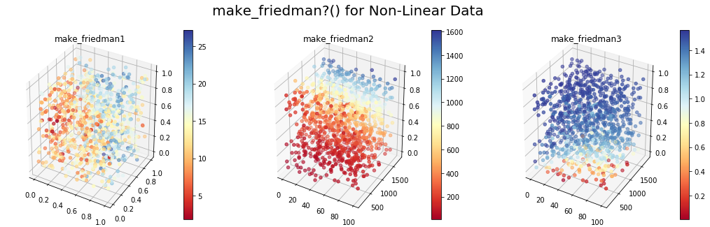
There are three versions of the make_friedman?() function (replace the ? with a value from {1,2,3}).
These functions generate the target variable using a non-linear combination of the input variables, as detailed below:
-
make_friedman1(): Then_featuresargument of this function has to be at least 5, hence generating a minimum number of 5 input dimensions. Here the target is given by:
$$
y(x) = 10 * \sin(\pi x_0 x_1) + 20(x_2 - 0.5)^2 + 10x_3 + 5x_4 + \text{noise}
$$ -
make_friedman2(): The generated data has 4 input dimensions. The response variable is given by:
$$
y(x) = \sqrt{(x_0^2+x_1 x_2 - \frac{1}{(x_1 x_3)^2})} + \text{noise}
$$
Check out our hands-on, practical guide to learning Git, with best-practices, industry-accepted standards, and included cheat sheet. Stop Googling Git commands and actually learn it!
make_friedman3(): The generated data in this case also has 4 dimensions. The output variable is given by:
$$
y(x) = \arctan(\frac{x_1 x_2 -\frac{1}{(x_1 x_3)}}{x_0})+\text{noise}
$$
The code below generates the datasets using these functions and plots the first three features in 3D, with colors varying according to the target variable:
fig = plt.figure(figsize=(18,5))

x,y = dt.make_friedman1(n_samples=1000,n_features=5,random_state=rand_state)
ax = fig.add_subplot(131, projection='3d')
my_scatter_plot = ax.scatter(x[:,0], x[:,1],x[:,2], c=y, cmap=color_map)
fig.colorbar(my_scatter_plot)
plt.title('make_friedman1')

x,y = dt.make_friedman2(n_samples=1000,random_state=rand_state)
ax = fig.add_subplot(132, projection='3d')
my_scatter_plot = ax.scatter(x[:,0], x[:,1],x[:,2], c=y, cmap=color_map)
fig.colorbar(my_scatter_plot)
plt.title('make_friedman2')

x,y = dt.make_friedman3(n_samples=1000,random_state=rand_state)
ax = fig.add_subplot(133, projection='3d')
my_scatter_plot = ax.scatter(x[:,0], x[:,1],x[:,2], c=y, cmap=color_map)
fig.colorbar(my_scatter_plot)
plt.suptitle('make_friedman?() for Non-Linear Data',fontsize=20)
plt.title('make_friedman3')

plt.show()
Synthetic Data for Classification
Scikit-learn has simple and easy-to-use functions for generating datasets for classification in the sklearn.dataset module. Let's go through a couple of examples.
make_classification() for n-Class Classification Problems
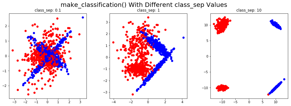
For n-class classification problems, the make_classification() function has several options:
class_sep: Specifies whether different classes should be more spread out and easier to discriminaten_features: Number of featuresn_redundant: Number of redundant featuresn_repeated: Number of repeated featuresn_classes: Total number of classes
Let's make a classification dataset for two-dimensional input data. We'll have different values of class_sep for a binary classification problem. The same colored points belong to the same class. It's worth noting that this function can also generate imbalanced classes:
fig,ax = plt.subplots(nrows=1, ncols=3,figsize=(16,5))
plt_ind_list = np.arange(3)+131

for class_sep,plt_ind in zip([0.1,1,10],plt_ind_list):
    x,y = dt.make_classification(n_samples=1000,
                                 n_features=2,
                                 n_repeated=0,
                                 class_sep=class_sep,
                                 n_redundant=0,
                                 random_state=rand_state)

    plt.subplot(plt_ind)
    my_scatter_plot = plt.scatter(x[:,0],
                                  x[:,1],
                                  c=y,
                                  vmin=min(y),
                                  vmax=max(y),
                                  s=35,
                                  cmap=color_map_discrete)
    plt.title('class_sep: '+str(class_sep))

fig.subplots_adjust(hspace=0.3,wspace=.3)
plt.suptitle('make_classification() With Different class_sep Values',fontsize=20)
plt.show()
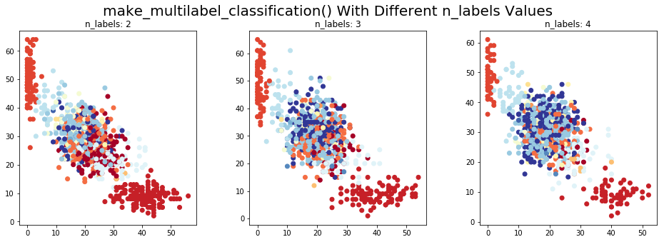
make_multilabel_classification() for Multi-Label classification problems
make_multilabel_classification() function generates data for multi-label classification problems. It has various options, of which the most notable one is n_label, which sets the average number of labels per data point.
Let's consider a 4-class multi-label problem, with the target vector of labels being converted to a single value for visualization. The points are colored according to the decimal representation of the binary label vector. The code will help you see how using a different value for n_label, changes the classification of a generated data point:
fig,ax = plt.subplots(nrows=1, ncols=3,figsize=(16,5))
plt_ind_list = np.arange(3)+131

for label,plt_ind in zip([2,3,4],plt_ind_list):
    x,y = dt.make_multilabel_classification(n_samples=1000,
                                            n_features=2,
                                            n_labels=label,
                                            n_classes=4,
                                            random_state=rand_state)
    target = np.sum(y*[8,4,2,1],axis=1)

    plt.subplot(plt_ind)
    my_scatter_plot = plt.scatter(x[:,0],
                                  x[:,1],
                                  c=target,
                                  vmin=min(target),
                                  vmax=max(target),
                                  cmap=color_map)
    plt.title('n_labels: '+str(label))

fig.subplots_adjust(hspace=0.3,wspace=.3)
plt.suptitle('make_multilabel_classification() With Different n_labels Values',fontsize=20)
plt.show()
Synthetic Data for Clustering
For clustering, the sklearn.datasets provides several options. Here, we'll cover the make_blobs() and make_circles() functions.
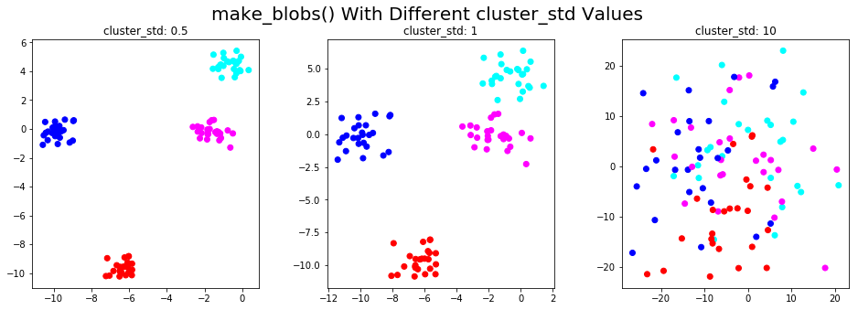
make_blobs()
The make_blobs() function generates data from isotropic Gaussian distributions. The number of features, the number of centers, and each cluster's standard deviation can be specified as an argument.
Here, we illustrate this function in 2D and show how data points change with different values of cluster_std parameter:
fig,ax = plt.subplots(nrows=1, ncols=3,figsize=(16,5))
plt_ind_list = np.arange(3)+131

for std,plt_ind in zip([0.5,1,10],plt_ind_list):
    x, label = dt.make_blobs(n_features=2,
                             centers=4,
                             cluster_std=std,
                             random_state=rand_state)

    plt.subplot(plt_ind)
    my_scatter_plot = plt.scatter(x[:,0],
                                  x[:,1],
                                  c=label,
                                  vmin=min(label),
                                  vmax=max(label),
                                  cmap=color_map_discrete)
    plt.title('cluster_std: '+str(std))

fig.subplots_adjust(hspace=0.3,wspace=.3)
plt.suptitle('make_blobs() With Different cluster_std Values',fontsize=20)
plt.show()
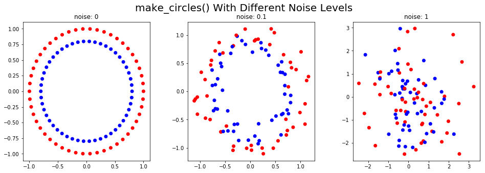
make_circles()
The make_circles() function generates two concentric circles with the same center, one within the other.
Using the noise parameter, distortion can be added to the generated data. This type of data is useful for evaluating affinity-based clustering algorithms. The code below shows the synthetic data generated at different noise levels:
fig,ax = plt.subplots(nrows=1, ncols=3,figsize=(16,5))
plt_ind_list = np.arange(3)+131

for noise,plt_ind in zip([0,0.1,1],plt_ind_list):
    x, label = dt.make_circles(noise=noise,random_state=rand_state)

    plt.subplot(plt_ind)
    my_scatter_plot = plt.scatter(x[:,0],
                                  x[:,1],
                                  c=label,
                                  vmin=min(label),
                                  vmax=max(label),
                                  cmap=color_map_discrete)
    plt.title('noise: '+str(noise))

fig.subplots_adjust(hspace=0.3,wspace=.3)
plt.suptitle('make_circles() With Different Noise Levels',fontsize=20)
plt.show()
Generating Samples Derived from an Input Dataset
There are many ways of generating additional data samples from an existing dataset. Here, we illustrate a very simple method that first estimates the kernel density of data using a Gaussian kernel and then generates additional samples from this distribution.
To visualize the newly generated samples, let's look at the Olivetti faces dataset, retrievable via sklearn.datasets.fetch_olivetti_faces(). The dataset has 10 different face images of 40 different people.
Here's what we'll be doing:
- Get the faces data
- Generate the kernel density model from data
- Use the kernel density to generate new samples of data
- Display the original and synthetic faces.
# Fetch the dataset and store in X
faces = dt.fetch_olivetti_faces()
X = faces.data

# Fit a kernel density model using GridSearchCV to determine the best parameter for bandwidth
bandwidth_params = {'bandwidth': np.arange(0.01,1,0.05)}
grid_search = GridSearchCV(KernelDensity(), bandwidth_params)
grid_search.fit(X)
kde = grid_search.best_estimator_

# Generate/sample 8 new faces from this dataset
new_faces = kde.sample(8, random_state=rand_state)

# Show a sample of 8 original face images and 8 generated faces derived from the faces dataset
fig,ax = plt.subplots(nrows=2, ncols=8,figsize=(18,6),subplot_kw=dict(xticks=[], yticks=[]))
for i in np.arange(8):
    ax[0,i].imshow(X[10*i,:].reshape(64,64),cmap=plt.cm.gray)
    ax[1,i].imshow(new_faces[i,:].reshape(64,64),cmap=plt.cm.gray)
ax[0,3].set_title('Original Data',fontsize=20)
ax[1,3].set_title('Synthetic Data',fontsize=20)
fig.subplots_adjust(wspace=.1)
plt.show()
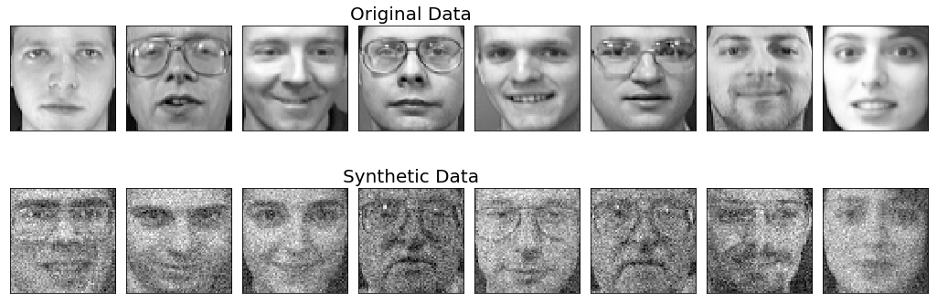
The original faces shown here are a sample of 8 faces chosen from 400 images, to get an idea of what the original dataset looks like. We can generate as many new data-points as we like using the sample() function.
In this example, 8 new samples were generated. Note that the synthetic faces shown here do not necessarily correspond to the face of the person shown above it.
Conclusions
In this article we got to know a few methods of generating synthetic datasets for various problems. Synthetic datasets help us evaluate our algorithms under controlled conditions and set a baseline for performance measures.
Python has a wide range of functions that can be used for artificial data generation. It is important to understand which functions and APIs can be used for your specific requirements.

