Implementing Other SVM Flavors with Python's Scikit-Learn

Introduction

This guide is the third and final part of three guides about Support Vector Machines (SVMs). In this guide, we will keep working with the forged bank notes use case, have a quick recap about the general idea behind SVMs, understand what is the kernel trick, and implement different types of non-linear kernels with Scikit-Learn.

In the complete series of SVM guides, besides learning about other types of SVMs, you will also learn about simple SVM, SVM pre-defined parameters, C and Gamma hyperparameters and how they can be tuned with grid search and cross validation.

If you wish to read the previous guides, you can take a look at the first two guides or see which topics interest you the most. Below is the table of topics covered in each guide:

1. Implementing SVM and Kernel SVM with Python's Scikit-Learn

• Use case: forget bank notes
• Background of SVMs
• Simple (Linear) SVM Model
  • About the Dataset
  • Importing the Dataset
  • Exploring the Dataset
• Implementing SVM with Scikit-Learn
  • Dividing Data into Train/Test Sets
  • Training the Model
  • Making Predictions
  • Evaluating the Model
  • Interpreting Results

2. Understanding SVM Hyperparameters

• The C Hyperparameter
• The Gamma Hyperparameter

3. Implementing other SVM flavors with Python's Scikit-Learn

• The General Idea of SVMs (a recap)
• Kernel (Trick) SVM
• Implementing Non-Linear Kernel SVM with Scikit-Learn
• Importing Libraries
  • Importing the Dataset
  • Dividing Data Into Features (X) and Target (y)
  • Dividing Data Into Train/Test Sets
  • Training the Algorithm
• Polynomial kernel
  • Making Predictions
  • Evaluating the Algorithm
• Gaussian kernel
  • Prediction and Evaluation
• Sigmoid Kernel
  • Prediction and Evaluation
• Comparison of Non-Linear Kernel Performances

Let's remember what SVM is all about before seeing some interesting SVM kernel variations.

The General Idea of SVMs

In case of linearly separable data in two dimensions (as shown in Fig. 1) the typical machine learning algorithm approach would be to try to find a boundary that divides the data in such a way that the misclassification error is minimized. If you look closely at figure 1, notice there can be several boundaries (infinite) that divide the data points correctly. The two dashed lines as well as the solid line are all valid classifications of the data.

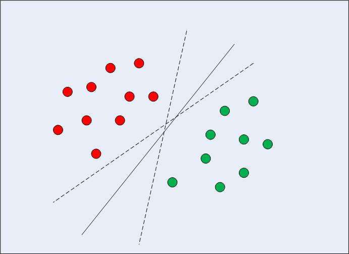
Fig 1: Multiple Decision Boundaries

When SVM chooses the decision boundary, it chooses a boundary that maximizes the distance between itself and the nearest data points of the classes. We already know that the nearest data points are the support vectors and that the distance can be parametrized both by C and gamma hyperparameters.

In calculating that decision boundary, the algorithm chooses how many points to consider and how far the margin can go - this configures a margin maximization problem. In solving that margin maximization problem, SVM uses the support vectors (as seen in Fig. 2) and tries to figure out what are optimal values that keep the margin distance bigger, while classifying more points correctly according to the function that is being used to separate the data.

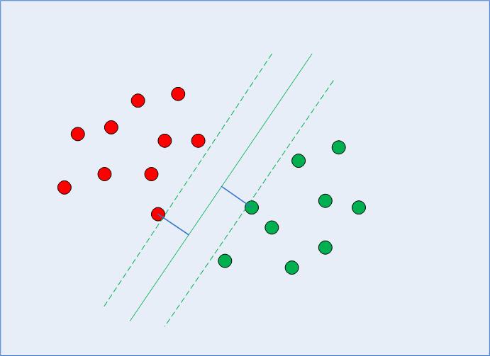
Fig 2: Decision Boundary with Support Vectors

This is why SVM differs from other classification algorithms, once it doesn't merely find a decision boundary, but it ends up finding the optimal decision boundary.

There is complex mathematics derived from statistics and computational methods involved behind finding the support vectors, calculating the margin between the decision boundary and the support vectors, and maximizing that margin. This time, we will not go into the details of how the mathematics play out.

It is always important to dive deeper and make sure machine learning algorithms are not some kind of mysterious spell, although not knowing every mathematical detail at this time didn't and won't stop you from being able to execute the algorithm and obtain results.

Kernel (Trick) SVM

In the previous section, we have remembered and organized the general idea of SVM - seeing how it can be used to find the optimal decision boundary for linearly separable data. However, in the case of non-linearly separable data, such as the one shown in Fig. 3, we already know that a straight line cannot be used as a decision boundary.

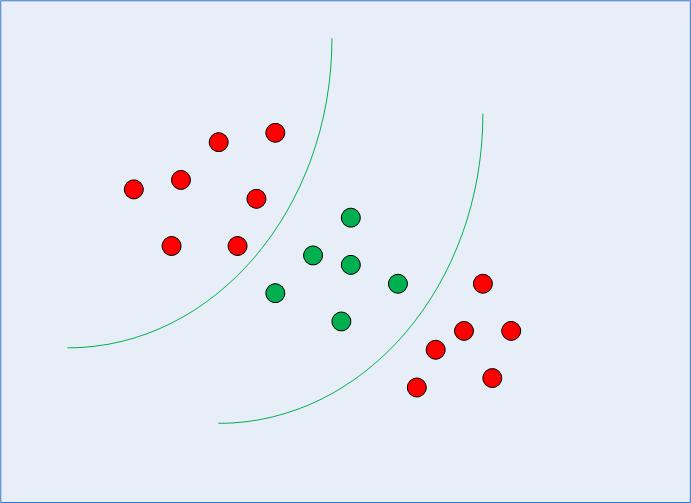
Fig 3: Non-linearly Separable Data

Rather, we can use the modified version of SVM we had discussed in the beginning, called Kernel SVM.

Basically, what the kernel SVM will do is to project the non-linearly separable data of lower dimensions to its corresponding form in higher dimensions. This is a trick, because when projecting non-linearly separable data in higher dimensions, the data shape changes in such a way that it becomes separable. For instance, when thinking about 3 dimensions, the data points from each class could end up being allocated in a different dimension, making it separable. One way of increasing the data dimensions can be through exponentiating it. Again, there is complex mathematics involved in this, but you do not have to worry about it in order to use SVM. Rather, we can use Python's Scikit-Learn library to implement and use the non-linear kernels in the same way we have used the linear.

Implementing Non-Linear Kernel SVM with Scikit-Learn

In this section, we will use the same dataset to predict whether a bank note is real or forged according to the four features we already know.

You will see that the rest of the steps are typical machine learning steps and need very little explanation until we reach the part where we train our Non-linear Kernel SVMs.

Importing Libraries

import numpy as np
import matplotlib.pyplot as plt
import pandas as pd
import seaborn as sns
from sklearn.model_selection import train_test_split

Importing the Dataset

data_link = "https://archive.ics.uci.edu/ml/machine-learning-databases/00267/data_banknote_authentication.txt"
col_names = ["variance", "skewness", "curtosis", "entropy", "class"]

bankdata = pd.read_csv(data_link, names=col_names, sep=",", header=None)
bankdata.head()mes)

Dividing Data Into Features (X) and Target (y)

X = bankdata.drop('class', axis=1)
y = bankdata['class']

Dividing Data into Train/Test Sets

SEED = 42

X_train, X_test, y_train, y_test = train_test_split(X, y, test_size = 0.20, random_state = SEED)

Training the Algorithm

To train the kernel SVM, we will use the same SVC class of the Scikit-Learn's svm library. The difference lies in the value for the kernel parameter of the SVC class.

In the case of the simple SVM we have used "linear" as the value for the kernel parameter. However, as we have mentioned earlier, for kernel SVM, we can use Gaussian, polynomial, sigmoid, or computable kernels. We will implement polynomial, Gaussian, and sigmoid kernels and look at its final metrics to see which one seems to fit our classes with a higher metric.

1. Polynomial kernel

In algebra, a polynomial is an expression of the form:

$$
2a*b^3 + 4a - 9
$$

This has variables, such as a and b, constants, in our example, 9 and coefficients (constants accompanied by variables), such as 2 and 4. The 3 is considered to be the degree of the polynomial.

There are types of data that can best be described when using a polynomial function, here, what the kernel will do is to map our data to a polynomial to which we will choose the degree. The higher the degree, the more the function will try to get closer to the data, so the decision boundary is more flexible (and more prone to overfit) - the lower the degree, the least flexible.

So, for implementing the polynomial kernel, besides choosing the poly kernel, we will also pass a value for the degree parameter of the SVC class. Below is the code:

from sklearn.svm import SVC
svc_poly = SVC(kernel='poly', degree=8)
svc_poly.fit(X_train, y_train)

Making Predictions

Now, once we have trained the algorithm, the next step is to make predictions on the test data.

As we have done before, we can execute the following script to do so:

y_pred_poly = svclassifier.predict(X_test)

Evaluating the Algorithm

As usual, the final step is to make evaluations on the polynomial kernel. Since we have repeated the code for the classification report and the confusion matrix a few times, let's transform it into a function that display_results after receiving the respective y_test, y_pred and title to the Seaborn's confusion matrix with cm_title:

def display_results(y_test, y_pred, cm_title):
    cm = confusion_matrix(y_test,y_pred)
    sns.heatmap(cm, annot=True, fmt='d').set_title(cm_title)
    print(classification_report(y_test,y_pred))

Now, we can call the function and look at the results obtained with the polynomial kernel:

cm_title_poly = "Confusion matrix with polynomial kernel"
display_results(y_test, y_pred_poly, cm_title_poly)

The output looks like this:

         precision    recall  f1-score   support

           0       0.69      1.00      0.81       148
           1       1.00      0.46      0.63       127

    accuracy                           0.75       275
   macro avg       0.84      0.73      0.72       275
weighted avg       0.83      0.75      0.73       275

Now we can repeat the same steps for Gaussian and sigmoid kernels.

2. Gaussian kernel

To use the gaussian kernel, we only need to specify rbf as value for the kernel parameter of the SVC class:

svc_gaussian = SVC(kernel='rbf', degree=8)
svc_gaussian.fit(X_train, y_train)

When further exploring this kernel, you can also use grid search to combine it with different C and gamma values.

Prediction and Evaluation

y_pred_gaussian = svc_gaussian.predict(X_test)

cm_title_gaussian = "Confusion matrix with Gaussian kernel"
display_results(y_test, y_pred_gaussian, cm_title_gaussian)

The output of the Gaussian kernel SVM looks like this:

                precision    recall  f1-score   support

           0       1.00      1.00      1.00       148
           1       1.00      1.00      1.00       127

    accuracy                           1.00       275
   macro avg       1.00      1.00      1.00       275
weighted avg       1.00      1.00      1.00       275

3. Sigmoid Kernel

Finally, let's use a sigmoid kernel for implementing Kernel SVM. Take a look at the following script:

svc_sigmoid = SVC(kernel='sigmoid')
svc_sigmoid.fit(X_train, y_train)

To use the sigmoid kernel, you have to specify 'sigmoid' as value for the kernel parameter of the SVC class.

Prediction and Evaluation

y_pred_sigmoid = svc_sigmoid.predict(X_test)

cm_title_sigmoid = "Confusion matrix with Sigmoid kernel"
display_results(y_test, y_pred_sigmoid, cm_title_sigmoid)

The output of the Kernel SVM with Sigmoid kernel looks like this:

                precision    recall  f1-score   support

           0       0.67      0.71      0.69       148
           1       0.64      0.59      0.61       127

    accuracy                           0.65       275
   macro avg       0.65      0.65      0.65       275
weighted avg       0.65      0.65      0.65       275

Comparison of Non-Linear Kernel Performances

If we briefly compare the performance of the different types of non-linear kernels, it might seem that the sigmoid kernel has the lowest metrics, so the worst performance.

Amongst the Gaussian and polynomial kernels, we can see that the Gaussian kernel achieved a perfect 100% prediction rate - which is usually suspicious and may indicate an overfit, while the polynomial kernel misclassified 68 instances of class 1.

Therefore, there is no hard and fast rule as to which kernel performs best in every scenario or in our current scenario without further searching for hyperparameters, understanding about each function shape, exploring the data, and comparing train and test results to see if the algorithm is generalizing.

It is all about testing all the kernels and selecting the one with the combination of parameters and data preparation that give the expected results according to the context of your project.

Conclusion

In this article we made a quick recap on SVMs, studied about the kernel trick and implemented different flavors of non-linear SVMs.

I suggest you implement each kernel and keep going further. You can explore the mathematics used to create each of the different kernels, why they were created and the differences regarding their hyperparameters. In that way, you will learn about the techniques and what type of kernel is best to apply depending on the context and the data available.

Having a clear understanding of how each kernel works and when to use them will definitely help you in your journey. Let us know how the progress is going and happy coding!