Stochastic Optimization: Random Search in Java

Introduction

Stochastic Optimization refers to a category of optimization algorithms that generate and utilize random points of data to find an approximate solution.

While brute-force algorithms do provide us with the best solution, they're terribly inefficient. This isn't an issue with smaller datasets, but most real-life problems and search-spaces require such a huge computational capability to be solved in a reasonable time-frame that such computers will likely exist beyond a predictable future.

In such cases, a new approach has to be used, and instead of searching for the actual best solution, we settle for an approximate solution that'll work good enough for us.

Many optimization methods exist, and each method can be implemented through many different algorithms. We'll start out by implementing the least efficient and most intuitive Stochastic Search algorithm - Random Search.

In pursuit of efficiency over absolute correctness, many random algorithms have been developed, culminating with evolutionary algorithms such as Genetic Algorithms.

Random Search

Random Search is the simplest stochastic search algorithm and it's very intuitive. For example, say we're searching for the maximum of a function. Instead of brute-forcing the solution, it generates random points on a dimension of the search space.

Then, it proceeds to check each of those points by comparing the current f_max against the value of the point it's on, assigning it a new value if necessary. After going through all the generated points, it returns us the f_max as the approximate solution.

The downside with all stochastic search algorithms, and especially Random Search, is that they can be as inefficient as brute-force algorithms if you don't balance it.

The more random points you use, the closer the approximation will be to the absolute best solution, but the slower the algorithm will be. With an infinite amount of random points, it's just a regular brute-force algorithm.

Here's a function generated by FooPlot as an example of how Random Search searches for the maximum/minimum of a function:

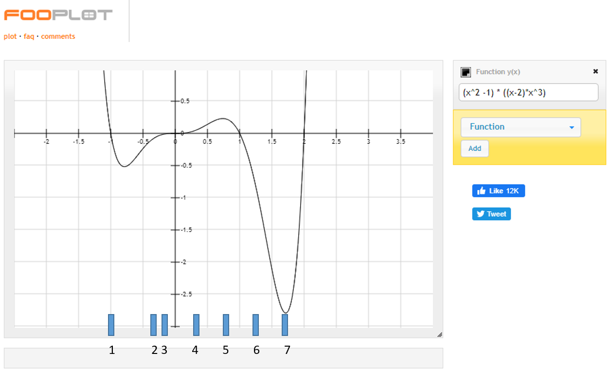
There are 7 randomly generated points here, where coincidentally the point 7 is located at the x value that will return the lowest y value and 5 is close to the value that will return the highest y value, for an example.

We'll limit the domain of the function to range from -1 to 2 and in that range, using simple high school calculus, it's easy to deduce that:

$$
f_{max} = (0.73947, 0.23098) \wedge f_{min} = (1.71548, -2.79090)
$$

That being said, depending on the specific accuracy you're looking for (95% for example), if Random Search approximates anything between (0.7, 0.2) and (0.75, 0.25) for the f_max and (1.65, -2.65) and (1.8, -2.9) for the f_min should be an approximately good solution.

Implementation

Let's go ahead and implement Random Search in Java. First, let's bound the domain of our function to {-1...2}:

private static final double START_DOMAIN = -1;
private static final double END_DOMAIN = 2;

Then, let's replicate the function from FooPlot, which of course, returns y based on x:

private double function(double x) {
    return ((Math.pow(x, 2)-1)*((x-2)*Math.pow(x, 3)));
}

Finally, let's implement the algorithm itself:

public void randomSearch() {
    double startPosition = START_DOMAIN;
    double maxY = function(startPosition);
    double maxX = START_DOMAIN;

    for (int i = 0; i < 10; i++) {
        double random = ThreadLocalRandom.current().nextDouble(START_DOMAIN, END_DOMAIN);

        if (function(random) > maxY) {
            maxY = function(random);
            maxX = random;
        }
    }

    System.out.println("The maximum of the function f(x) is (" + maxX + ", " + maxY + ")");
}

The starting position for the iteration is obviously at the start of the domain. The maxY is calculated using the function() method we've defined and the maxX is set as the value at the start of the domain as well.

These are the current max values as we haven't evaluated anything else yet. As soon as we assign them the default values, through a for loop, we generate a random point between the start and the end of the domain. We then evaluate if the random point, passed through the function(), is by any change larger than the current maxY.

Note: We're using a ThreadLocalRandom instead of a regular Random since ThreadLocalRandom can work way faster than Random in a multi-threaded environment. In our case, it doesn't make much of a difference, but it can make a significant one. Also, it's easier to define a range of doubles using ThreadLocalRandom.

If it is, the maxY is set to the function(random) as it returns the y value and the maxX is set to the random as that's the one that produced the largest y value through the function() method.

After the for loop terminates, we're left with maxX and maxY with certain values, which are essentially an approximation of what the actual maximum x and y are.

Running this piece of code will yield:

The maximum of the function f(x) is (0.7461978805972576, 0.2308765022939988)

And comparing this to the actual results, it's pretty accurate, with a measly 10 random points. If we increase the number of random points from 10 to 100, we get the following result:

The maximum of the function f(x) is (0.735592753214972, 0.2309513390409203)

There's not a lot of improvement between the two, which just goes to show that 100 iterations is completely unneeded. If we take the liberty of reducing it from 10 to 5, we'll see that's it's off:

The maximum of the function f(x) is (0.6756978982704229, 0.22201906058201992)

Again, depending on your accuracy needs, this might just be an acceptable solution.

Changing the algorithm to search for a minimum instead of the maximum is as easy as changing the > operator to a < operator in the if clause.

Conclusion

Sometimes, an approximation of the solution is good enough for your needs and you don't need to force your machine to find the best possible solution.

This approach is extremely useful when you're dealing with problems of huge computational complexity and can improve the performance of your program by orders of magnitude.

Of course, if you don't balance the algorithm right, you'll end up with an inefficient solution, so play around with the number of random points in order to get an efficient one.!