Creating a Neural Network from Scratch in Python: Adding Hidden Layers

This is the second article in the series of articles on "Creating a Neural Network From Scratch in Python".

• Creating a Neural Network from Scratch in Python
• Creating a Neural Network from Scratch in Python: Adding Hidden Layers
• Creating a Neural Network from Scratch in Python: Multi-class Classification

If you are absolutely beginner to neural networks, you should read Part 1 of this series first (linked above). Once you are comfortable with the concepts explained in that article, you can come back and continue with this article.

Introduction

In the previous article, we started our discussion about artificial neural networks; we saw how to create a simple neural network with one input and one output layer, from scratch in Python. Such a neural network is called a perceptron. However, real-world neural networks, capable of performing complex tasks such as image classification and stock market analysis, contain multiple hidden layers in addition to the input and output layer.

In the previous article, we concluded that a Perceptron is capable of finding linear decision boundary. We used perceptron to predict whether a person is diabetic or not using a toy dataset. However, a perceptron is not capable of finding non-linear decision boundaries.

In this article, we will build upon the concepts that we studied in Part 1 of this series and will develop a neural network with one input layer, one hidden layer, and one output layer. We will see that the neural network that we will develop will be capable of finding non-linear boundaries.

Dataset

For this article, we need non-linearly separable data. In other words, we need a dataset that cannot be classified using a straight line.

Luckily, Python's Scikit Learn library comes with a variety of tools that can be used to automatically generate different types of datasets.

Execute the following script to generate the dataset that we are going to use, in order to train and test our neural network.

from sklearn import datasets

np.random.seed(0)
feature_set, labels = datasets.make_moons(100, noise=0.10)
plt.figure(figsize=(10,7))
plt.scatter(feature_set[:,0], feature_set[:,1], c=labels, cmap=plt.cm.winter)

In the script above we import the datasets class from the sklearn library. To create non-linear dataset of 100 data-points, we use the make_moons method and pass it 100 as the first parameter. The method returns a dataset, which when plotted contains two interleaving half circles, as shown in the figure below:

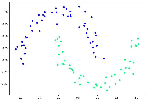
You can clearly see that this data cannot be separated by a single straight line, hence the perceptron cannot be used to correctly classify this data.

Let's verify this concept. To do so, we'll use a simple perceptron with one input layer and one output layer (the one we created in the last article) and try to classify our "moons" dataset. Execute the following script:

from sklearn import datasets
import numpy as np
import matplotlib.pyplot as plt

np.random.seed(0)
feature_set, labels = datasets.make_moons(100, noise=0.10)
plt.figure(figsize=(10,7))
plt.scatter(feature_set[:,0], feature_set[:,1], c=labels, cmap=plt.cm.winter)

labels = labels.reshape(100, 1)

def sigmoid(x):
    return 1/(1+np.exp(-x))

def sigmoid_der(x):
    return sigmoid(x) *(1-sigmoid (x))

np.random.seed(42)
weights = np.random.rand(2, 1) 
lr = 0.5
bias = np.random.rand(1)

for epoch in range(200000):
    inputs = feature_set

    # feedforward step 1
    XW = np.dot(feature_set,weights) + bias

    # feedforward step 2
    z = sigmoid(XW)

    # backpropagation step 1
    error_out = ((1 / 2) * (np.power((z - labels), 2)))
    print(error_out.sum())

    error = z - labels

    # backpropagation step 2
    dcost_dpred = error
    dpred_dz = sigmoid_der(z) 

    z_delta = dcost_dpred * dpred_dz

    inputs = feature_set.T
    weights -= lr * np.dot(inputs, z_delta)

    for num in z_delta:
        bias -= lr * num

You will see that the value of mean squared error will not converge beyond 4.17 percent, no matter what you do. This indicates to us that we can't possibly correctly classify all points of the dataset using this perceptron, no matter what we do.

Neural Networks with One Hidden Layer

In this section, we will create a neural network with one input layer, one hidden layer, and one output layer. The architecture of our neural network will look like this:

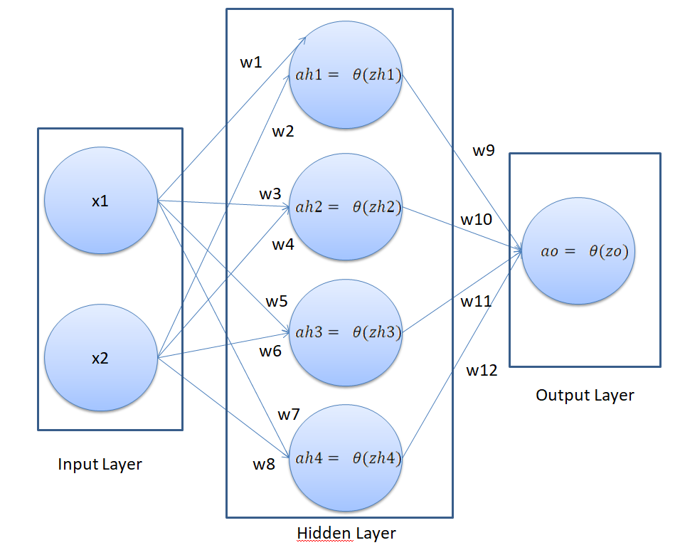
In the figure above, we have a neural network with 2 inputs, one hidden layer, and one output layer. The hidden layer has 4 nodes. The output layer has 1 node since we are solving a binary classification problem, where there can be only two possible outputs. This neural network architecture is capable of finding non-linear boundaries.

No matter how many nodes and hidden layers are there in the neural network, the basic working principle remains the same. You start with the feed-forward phase where inputs from the previous layer are multiplied with the corresponding weights and are passed through the activation function to get the final value for the corresponding node in the next layer. This process is repeated for all the hidden layers until the output is calculated. In the back-propagation phase, the predicted output is compared with the actual output and the cost of error is calculated. The purpose is to minimize the cost function.

This is pretty straight-forward if there is no hidden layer involved as we saw in the previous article.

However, if one or more hidden layers are involved, the process becomes a bit more complex because the error has to be propagated back to more than one layer since weights in all the layers are contributing towards the final output.

In this article, we will see how to perform feed-forward and back-propagation steps for the neural network having one or more hidden layers.

Feed Forward

For each record, we have two features "x1" and "x2". To calculate the values for each node in the hidden layer, we have to multiply the input with the corresponding weights of the node for which we are calculating the value. We then pass the dot product through an activation function to get the final value.

For instance to calculate the final value for the first node in the hidden layer, which is denoted by "ah1", you need to perform the following calculation:

$$
zh1 = x1w1 + x2w2
$$

$$
ah1 = \frac{\mathrm{1} }{\mathrm{1} + e^{-zh1} }
$$

This is the resulting value for the top-most node in the hidden layer. In the same way, you can calculate the values for the 2nd, 3rd, and 4th nodes of the hidden layer.

Similarly, to calculate the value for the output layer, the values in the hidden layer nodes are treated as inputs. Therefore, to calculate the output, multiply the values of the hidden layer nodes with their corresponding weights and pass the result through an activation function.

This operation can be mathematically expressed by the following equation:

$$
zo = ah1w9 + ah2w10 + ah3w11 + ah4w12
$$

$$
a0 = \frac{\mathrm{1} }{\mathrm{1} + e^{-z0} }
$$

Here "a0" is the final output of our neural network. Remember that the activation function that we are using is the sigmoid function, as we did in the previous article.

Note: For the sake of simplicity, we did not add a bias term to each weight. You will see that the neural network with the hidden layer will perform better than the perceptron, even without the bias term.

Back Propagation

The feed forward step is relatively straight-forward. However, the back-propagation is not as straight-forward as it was in Part 1 of this series.

In the back-propagation phase, we will first define our loss function. We will be using the mean squared error cost function. It can be represented mathematically as:

$$
MSE =
\frac{\mathrm{1} }{\mathrm{n}}
\sum\nolimits_{i=1}^{n}
(predicted - observed)^{2}
$$

Here n is the number of observations.

Phase 1

In the first phase of back propagation, we need to update weights of the output layer i.e w9, w10, w11, and w12. So for the time being, just consider that our neural network has the following part:

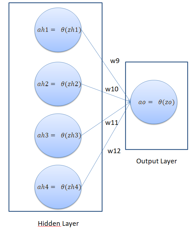
This looks similar to the perceptron that we developed in the last article. The purpose of the first phase of back propagation is to update weights w9, w10, w11, and w12 in such a way that the final error is minimized. This is an optimization problem where we have to find the function minima for our cost function.

To find the minima of a function, we can use the gradient decent algorithm. The gradient descent algorithm can be mathematically represented as follows:

The details regarding how gradient descent function minimizes the cost have already been discussed in the previous article. Here we'll just see the mathematical operations that we need to perform.

Our cost function is:

$$
MSE = \frac{\mathrm{1} }{\mathrm{n}} \sum\nolimits_{i=1}^{n}(predicted - observed)^{2}
$$

In our neural network, the predicted output is represented by "ao". Which means that we have to basically minimize this function:

$$
cost = \frac{\mathrm{1} }{\mathrm{n}} \sum\nolimits_{i=1}^{n}(ao - observed)^{2}
$$

From the previous article, we know that to minimize the cost function, we have to update weight values such that the cost decreases. To do so, we need to take derivative of the cost function with respect to each weight. Since in this phase, we are dealing with weights of the output layer, we need to differentiate cost function with respect to w9, w10, w11, and w2.

The differentiation of the cost function with respect to weights in the output layer can be mathematically represented as follows using the chain rule of differentiation.

$$
\frac {dcost}{dwo} = \frac {dcost}{dao} *, \frac {dao}{dzo} * \frac {dzo}{dwo} ...... (1)
$$

Here "wo" refers to the weights in the output layer. The letter "d" at the start of each term refers to “derivative”.

Let's find the value for each expression in Equation 1.

Here,

$$
\frac {dcost}{dao} = \frac {2}{n} * (ao - labels)
$$

Here 2 and n are constant. If we ignore them, we have the following equation.

$$
\frac {dcost}{dao} = (ao - labels) ........ (5)
$$

Next, we can find "dao" with respect to "dzo" as follows:

$$
\frac {dao}{dzo} = sigmoid(zo) * (1-sigmoid(zo)) ........ (6)
$$

Finally, we need to find "dzo" with respect to "dwo". The derivative is simply the inputs coming from the hidden layer as shown below:

$$
\frac {dzo}{dwo} = ah
$$

Here "ah" refers to the 4 inputs from the hidden layers. Equation 1 can be used to find the updated weight values for the weights for the output layer. To find new weight values, the values returned by Equation 1 can be simply multiplied with the learning rate and subtracted from the current weight values. This is straightforward and we have done this previously.

Phase 2

In the previous section, we saw how we can find the updated values for the output layer weights i.e. w9, w10, w11, and 12. In this section, we will back-propagate our error to the previous layer and find the new weight values for hidden layer weights i.e. weights w1 to w8.

Let's collectively denote hidden layer weights as "wh". We basically have to differentiate the cost function with respect to "wh". Mathematically we can use chain rule of differentiation to represent it as:

$$
\frac {dcost}{dwh} = \frac {dcost}{dah} *, \frac {dah}{dzh} * \frac {dzh}{dwh} ...... (2)
$$

Here again we will break Equation 2 into individual terms.

The first term "dcost" can be differentiated with respect to "dah" using the chain rule of differentiation as follows:

$$
\frac {dcost}{dah} = \frac {dcost}{dzo} *, \frac {dzo}{dah} ...... (3)
$$

Let's again break the Equation 3 into individual terms. Using the chain rule again, we can differentiate "dcost" with respect to "dzo" as follows:

$$
\frac {dcost}{dzo} = \frac {dcost}{dao} *, \frac {dao}{dzo} ...... (4)
$$

We have already calculated the value of dcost/dao in Equation 5 and dao/dzo in _Equation 6 _.

Now we need to find dzo/dah from Equation 3. If we look at zo, it has the following value:

$$
zo = a01w9 + a02w10 + a03w11 + a04w12
$$

If we differentiate it with respect to all inputs from the hidden layer, denoted by "ao", then we are left with all the weights from the output layer, denoted by "wo". Therefore,

$$
\frac {dzo}{dah} = wo ...... (7)
$$

Now we can find the value of dcost/dah by replacing the values from Equations 7 and 4 in Equation 3.

Coming back to Equation 2, we have yet to find dah/dzh and dzh/dwh.

The first term dah/dzh can be calculated as:

$$
\frac {dah}{dzh} = sigmoid(zh) * (1-sigmoid(zh)) ........ (8)
$$

And finally, dzh/dwh is simply the input values:

$$
\frac {dzh}{dwh} = input features ........ (9)
$$

If we replace the values from Equations 3, 8 and 9 in Equation 3, we can get the updated matrix for the hidden layer weights. To find new weight values for the hidden layer weights "wh", the values returned by Equation 2 can be simply multiplied with the learning rate and subtracted from the current weight values. And that's pretty much it.

The equations may look exhausting to you since there are a lot of calculations being performed. However, if you look at them closely, there are just two operations being performed in a chain: derivations and multiplications.

One of the reasons that neural networks are slower than the other machine learning algorithms is the fact that lots of computations are being performed at the back end. Our neural network had just one hidden layer with four nodes, two inputs and one output, yet we had to perform lengthy derivation and multiplication operations, in order to update the weights for a single iteration. In the real world, neural networks can have hundreds of layers with hundreds of inputs and output values. Therefore, neural networks execute slowly.

Code for Neural Networks with One Hidden Layer

Now let's implement the neural network that we just discussed in Python from scratch. You will clearly see the correspondence between the code snippets and the theory that we discussed in the previous section. We will again try to classify the non-linear data that we created in the Dataset section of the article. Take a look at the following script.

# -*- coding: utf-8 -*-
"""
Created on Tue Sep 25 13:46:08 2018

@author: usman
"""

from sklearn import datasets
import numpy as np
import matplotlib.pyplot as plt

np.random.seed(0)
feature_set, labels = datasets.make_moons(100, noise=0.10)
plt.figure(figsize=(10,7))
plt.scatter(feature_set[:,0], feature_set[:,1], c=labels, cmap=plt.cm.winter)

labels = labels.reshape(100, 1)

def sigmoid(x):
    return 1/(1+np.exp(-x))

def sigmoid_der(x):
    return sigmoid(x) *(1-sigmoid (x))

wh = np.random.rand(len(feature_set[0]),4) 
wo = np.random.rand(4, 1)
lr = 0.5

for epoch in range(200000):
    # feedforward
    zh = np.dot(feature_set, wh)
    ah = sigmoid(zh)

    zo = np.dot(ah, wo)
    ao = sigmoid(zo)

    # Phase1 =======================

    error_out = ((1 / 2) * (np.power((ao - labels), 2)))
    print(error_out.sum())

    dcost_dao = ao - labels
    dao_dzo = sigmoid_der(zo) 
    dzo_dwo = ah

    dcost_wo = np.dot(dzo_dwo.T, dcost_dao * dao_dzo)

    # Phase 2 =======================

    # dcost_w1 = dcost_dah * dah_dzh * dzh_dw1
    # dcost_dah = dcost_dzo * dzo_dah
    dcost_dzo = dcost_dao * dao_dzo
    dzo_dah = wo
    dcost_dah = np.dot(dcost_dzo , dzo_dah.T)
    dah_dzh = sigmoid_der(zh) 
    dzh_dwh = feature_set
    dcost_wh = np.dot(dzh_dwh.T, dah_dzh * dcost_dah)

    # Update Weights ================

    wh -= lr * dcost_wh
    wo -= lr * dcost_wo

In the script above we start by importing the desired libraries and then we create our dataset. Next, we define the sigmoid function along with its derivative. We then initialize the hidden layer and output layer weights with random values. The learning rate is 0.5. I tried different learning rates and found that 0.5 is a good value.

We then execute the algorithm for 2000 epochs. Inside each epoch, we first perform the feed-forward operation. The code snippet for the feed forward operation is as follows:

zh = np.dot(feature_set, wh)
ah = sigmoid(zh)

zo = np.dot(ah, wo)
ao = sigmoid(zo)

As discussed in theory section, back propagation consists of two phases. In the first phase, the gradients for the output layer weights are calculated. The following script executes in the first phase of the back-propagation.

error_out = ((1 / 2) * (np.power((ao - labels), 2)))
print(error_out.sum())

dcost_dao = ao - labels
dao_dzo = sigmoid_der(zo) 
dzo_dwo = ah

dcost_wo = np.dot(dzo_dwo.T, dcost_dao * dao_dzo)

In the second phase, the gradients for the hidden layer weights are calculated. The following script executes in the second phase of the back-propagation.

dcost_dzo = dcost_dao * dao_dzo
dzo_dah = wo
dcost_dah = np.dot(dcost_dzo , dzo_dah.T)
dah_dzh = sigmoid_der(zh) 
dzh_dwh = feature_set
dcost_wh = np.dot( dzh_dwh.T, dah_dzh * dcost_dah)

Finally, the weights are updated in the following script:

wh -= lr * dcost_wh
wo -= lr * dcost_wo

When the above script executes, you will see a minimum mean squared error value of 1.50 which is less than our previous mean squared error of 4.17, which was obtained using the perceptron. This shows that the neural network with hidden layers performs better in the case of non-linearly separable data.

Conclusion

In this article, we saw how we can create a neural network with 1 hidden layer, from scratch in Python. We saw how our neural network outperformed a neural network with no hidden layers for the binary classification of non-linear data.

However, we may need to classify data into more than two categories. In our next article, we will see how to create a neural network from scratch in Python for multi-class classification problems.